数据处理（三）| 深入数据预处理：提升机器学习模型性能的关键步骤

原创

CoovallyAIHub

发布于 2025-03-03 16:48:33

12100

代码可运行

运行总次数：0

代码可运行

今天要和大家继续讲解机器学习中一个看似枯燥但至关重要的环节——数据预处理。前面已经讲解过数据清洗和数据评质量评估（点击跳转），如果你已看过，那你已经打下了坚实的基础！今天这篇内容会更聚焦于预处理的核心技巧，手把手教你如何将原始数据“打磨”成模型的最爱。

一、为什么数据预处理是“模型的命门”？

如果你要训练一个猫狗模型，但给你的数据中：有的图片亮度忽明忽暗（尺度不一致），有的标签写着“猫”却混入了狗的照片（噪声干扰），甚至有些图片只有半只猫（数据缺失），这样的数据直接丢给模型，结果只能是检测效果大打折扣！数据预处理可以解释为数据清洗和数据评估等的总和，其中还包括数据转换等，所以它们的目标都是一致的

数据预处理的核心目标：

让数据更“干净”（解决缺失、噪声、重复等问题）；
让数据更“规范”（统一尺度、格式）；
让数据更“聪明”（通过特征工程挖掘隐藏信息）。

小贴士：数据清洗和评估的详细操作，可以回顾我们之前的文章哦～

二、数据预处理的核心步骤

处理缺失值

缺失值可能导致模型训练失败或结果偏差。常出现在用户年龄缺失、商品价格为空、传感器数据断档。常见的处理方法包括：

均值填充：适用于数值型数据，但对离群值敏感。
中位数填充：适合存在离群值的数据。
众数填充：适用于类别型数据。
删除缺失值：当缺失样本较少且不影响整体分布时，可直接删除。

代码示例（使用SimpleImputer方法填充缺失值）：

import pandas as pd
from sklearn.impute import SimpleImputer

df = pd.read_csv('./file/data.csv')
print(df)

# 填充缺失值
# {"constant", "mean", "median", "most_frequent"}
imputer = SimpleImputer(strategy='most_frequent')
df_imputed = imputer.fit_transform(df)

print(df_imputed)

数据缩放

机器学习算法对特征尺度敏感，比如假设身高（单位：米）和体重（单位：公斤）两个特征，数值范围差异巨大，模型会误认为体重更重要！所以需统一数据范围：

标准化（Standardization）：将数据转换为均值为0、标准差为1的分布，适用于KNN、SVM等基于距离的算法。

import pandas as pd
from sklearn.preprocessing import StandardScaler

X = pd.DataFrame({
    'x1': [1, 2, 3],
    'x2': [4, 5, 6],
    'x3': [7, 8, 9]
})
print(X)

# 标准化
scaler = StandardScaler()
X_scaled = scaler.fit_transform(X)
print(X_scaled)

归一化（Normalization）：将数据缩放到[0,1]区间，适合神经网络等梯度优化算法。

import pandas as pd
from sklearn.preprocessing import MinMaxScaler

X = pd.DataFrame({
    'x1': [1, 2, 3],
    'x2': [4, 5, 6],
    'x3': [7, 8, 9]
})
print(X)

# 归一化
scaler = MinMaxScaler()
X_scaled = scaler.fit_transform(X)
print(X_scaled)

测试集要用训练集的均值和标准差，避免数据泄漏！类别型特征不需要缩放，但需要编码（见下一部分）

类别变量编码

模型无法直接处理字符串类别，需转换为数值形式：

标签编码（Label Encoding）：为有序类别分配整数标签（如“低、中、高”）映射为0/1/2。

from sklearn.preprocessing import LabelEncoder

y = ['cat', 'dog', 'cat', 'bird', 'dog']

# 创建标签编码器
le = LabelEncoder()
# 对类别数据进行编码
y_encoded = le.fit_transform(y)
print(y_encoded)

独热编码（One-Hot Encoding）：为无序类别生成二进制向量（如颜色、国家）。

import numpy as np
from sklearn.preprocessing import OneHotEncoder

y = ['cat', 'dog', 'cat', 'bird', 'dog']

# 创建独热编码器
ohe = OneHotEncoder(sparse_output=False)
# 对类别数据进行编码
y_encoded = ohe.fit_transform(np.array(y).reshape(-1, 1))
print(y_encoded)

注意：类别过多时（如用户ID），独热编码会导致维度爆炸，建议用特征哈希或嵌入（Embedding）。

特征选择与工程

特征工程通过组合、转换现有特征，甚至创造新特征，让数据更贴合模型需求。

递归特征消除（RFE）：逐步剔除不重要的特征。

import numpy as np
import pandas as pd
from sklearn.feature_selection import RFE
from sklearn.ensemble import RandomForestClassifier
from sklearn.model_selection import train_test_split


# 生成一些示例数据
np.random.seed(42)
X = np.random.rand(200, 5) # 200个样本，5个特征
y = np.random.randint(0, 2, size=200) # 二分类标签

# 划分训练集和测试集
X_train, X_test, y_train, y_test = train_test_split(X, y, test_size=0.2, random_state=42)
column_names = [f"Feature_{i+1}" for i in range(X.shape[1])]
X_train = pd.DataFrame(X_train, columns=column_names)

# 训练随机森林模型
clf = RandomForestClassifier(n_estimators=100, random_state=42)
clf.fit(X_train, y_train)

# 递归特征消除
rfe = RFE(clf, n_features_to_select=3) # 选择前3个最重要的特征
X_rfe = rfe.fit_transform(X_train, y_train)

# 输出选择的特征
selected_features = X_train.columns[rfe.support_]
print("Selected features:", selected_features)

基于模型的重要性评估：利用随机森林、决策树等模型筛选关键特征。

import numpy as np
from sklearn.ensemble import RandomForestClassifier
from sklearn.model_selection import train_test_split

# 生成一些示例数据
X = np.random.rand(100, 2)#100个样本，2个特征
y = (X[:, 0]>X[:, 1]).astype(int) # 根据第一个特征是否大于第二个特征生成标签

# 划分训练集和测试集
X_train, X_test, y_train, y_test = train_test_split(X, y, test_size=0.2, random_state=42)

# 创建随机森林分类器
clf = RandomForestClassifier()
clf.fit(X_train, y_train)

# 获取特征重要性
feature_importances = clf.feature_importances_
print(feature_importances)

组合特征：如将“身高”和“体重”组合为“BMI”。
时间特征提取：从时间戳中提取“月份”“星期”等。
主成分分析（PCA）：通过线性变换将数据从高维空间映射到低维空间，使得新特征（主成分）尽可能保留数据的方差，特别适用于特征数量过多的情况，可以有效降低计算复杂度。

import numpy as np
from sklearn.decomposition import PCA
from sklearn.preprocessing import StandardScaler


# 生成一个特征矩阵
np.random.seed(0)
X = np.random.rand(100, 5) # 100个样本，每个样本5个特征

# 数据预处理：标准化特征矩阵
scaler = StandardScaler()
X_scaled = scaler.fit_transform(X)

# 应用PCA降维到2个主成分
pca = PCA(n_components=2)
X_pca = pca.fit_transform(X_scaled)

# 打印每个主成分的方差解释比例
print("Explained Variance Ratio:", pca.explained_variance_ratio_)

线性判别分析（LDA）:LDA是一种监督学习的降维方法，通常用于分类任务中，它旨在找到一个线性组合，使得不同类别之间的距离最大化，类别内的距离最小化。

import numpy as np
from sklearn.discriminant_analysis import LinearDiscriminantAnalysis
from sklearn.preprocessing import StandardScaler


# 假设X是特征矩阵，y是目标变量，这里我们使用随机数据来模拟
np.random.seed(0)
X = np.random.rand(100, 5)  # 100个样本，每个样本5个特征
y = np.random.randint(0, 3, 100)  # 100个样本的目标变量，0、1或2

# 数据预处理：标准化特征矩阵
scaler = StandardScaler()
X_scaled = scaler.fit_transform(X)

# 检查类别数量
n_classes = len(np.unique(y))
print("Number of unique classes:", n_classes)

# 确定n_components的值
n_features = X_scaled.shape[1]
n_components = min(2, n_features, n_classes - 1) # 确保n_components不超过2、特征数和类别数-1的最小值
print("Number of components:", n_components)

# 应用LDA降维
lda = LinearDiscriminantAnalysis(n_components=n_components)
X_lda = lda.fit_transform(X_scaled, y)

# 输出降维后的数据
print(X_lda)

处理不平衡数据

类别样本不均衡会导致模型偏向多数类，解决方法包括：

上采样（Over-sampling）：使用SMOTE算法生成少数类样本。

import numpy as np
from imblearn.over_sampling import SMOTE


# 生成测试数据
np.random.seed(0)
X_train = np.random.rand(100, 5) # 100个样本，每个样本5个特征
y_train = np.random.randint(0, 2, 100) # 随机生成100个类别标签，0或1

# 检查类别平衡
print("Original dataset shape:", X_train.shape)
print("Original labels count:", np.bincount(y_train))

# 初始化SMOTE对象
smote = SMOTE()

# 拟合并重采样数据
X_resampled, y_resampled = smote.fit_resample(X_train, y_train)

# 检查重采样后的数据
print("Resampled dataset shape:", X_resampled.shape)
print("Resampled labels count:", np.bincount(y_resampled))

下采样（Under-sampling）：随机减少多数类样本。

import numpy as np
from imblearn.under_sampling import RandomUnderSampler

# 生成测试数据
np.random.seed(0)
X_train = np.random.rand(100, 5) # 100个样本，每个样本5个特征
y_train = np.random.randint(0, 2, 100) # 随机生成100个类别标签，0或1

# 检查类别平衡
print("Original dataset shape:", X_train.shape)
print("Original labels count:", np.bincount(y_train))

# 初始化下采样对象
undersampler = RandomUnderSampler()

# 拟合并重采样数据
X_resampled, y_resampled = undersampler.fit_resample(X_train, y_train)

# 检查重采样后的类别平衡
print("Resampled dataset shape:", X_resampled.shape)
print("Resampled labels count:", np.bincount(y_resampled))

三、工具加持：NumPy & Pandas高效技巧

NumPy：科学计算基础

NumPy是Python中高效处理数值计算的基础库，核心是多维数组（ndarray），比Python原生列表快百倍！

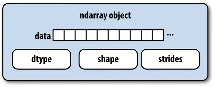
数组操作：支持高效的多维数组（ndarray）运算。

创建数组：从列表到矩阵

import numpy as np  

# 一维数组  
arr1d = np.array([1, 2, 3, 4])  

# 二维数组（矩阵）  
arr2d = np.array([[1, 2], [3, 4]])  

# 特殊数组：零矩阵、单位矩阵  
zeros = np.zeros((3, 3))    # 3x3零矩阵  
ones = np.ones((2, 4))      # 2x4全1矩阵  
identity = np.eye(3)        # 3x3单位矩阵

数组操作：切片、筛选、变形

# 切片（前两行，第二列）  
subset = arr2d[:2, 1]  

# 条件筛选（大于2的值）  
mask = arr1d > 2  
filtered = arr1d[mask]  

# 改变形状（2x2矩阵转为4x1向量）  
reshaped = arr2d.reshape(4, 1)

广播机制：自动扩展不同形状数组的运算。

场景：计算矩阵每行的均值并中心化。

matrix = np.array([[1, 2, 3], [4, 5, 6], [7, 8, 9]])  
row_means = matrix.mean(axis=1, keepdims=True)  # 保持维度，便于广播  
centered_matrix = matrix - row_means

广播规则：

从后往前对齐维度，缺失的维度自动补1。

任一维度长度为1时，可扩展至另一数组对应维度长度。

高效条件筛选：np.where的妙用

场景：将数据中的异常值替换为阈值。

data = np.array([10, 20, 30, 100, 5, 200])  
cleaned_data = np.where(data > 50, 50, data)  # 大于50的值替换为50

进阶技巧：结合逻辑运算符（&、|、~）实现复杂条件。

内存优化：避免不必要的数组复制

陷阱：切片操作可能产生视图（view）或副本（copy），影响性能。

验证方法：

arr = np.arange(10)  
view = arr[3:6]  
view.base is arr  # 返回True，说明是视图  
copy = arr[3:6].copy()  
copy.base is None  # 返回True，说明是副本

优化原则：尽量使用视图操作，减少内存占用。

Pandas：数据分析利器

Pandas是专为结构化数据设计的库，核心是DataFrame（二维表格）和Series（一维序列），让数据清洗和分析变得像Excel一样简单

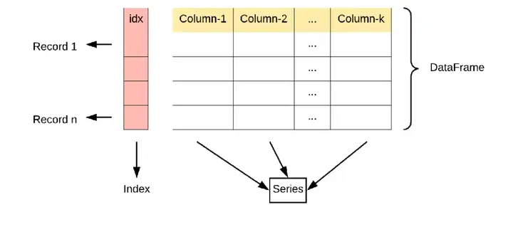
Series：一维带标签数组，支持自动对齐。

DataFrame：二维表格，支持灵活的数据操作（排序、聚合、清洗）。

创建DataFrame：从字典到表格

import pandas as pd  

# 从字典创建  
data = {  
    '姓名': ['张三', '李四', '王五'],  
    '年龄': [25, 30, 28],  
    '城市': ['北京', '上海', '深圳']  
}  
df = pd.DataFrame(data)  

# 输出结果：
#    姓名  年龄  城市  
# 0 张三  25  北京  
# 1 李四  30  上海  
# 2 王五  28  深圳

数据操作：查询、排序、聚合

# 查询年龄大于26岁的人  
df_filtered = df[df['年龄'] > 26]  

# 按城市分组计算平均年龄  
df_grouped = df.groupby('城市')['年龄'].mean()  

# 按年龄排序  
df_sorted = df.sort_values('年龄', ascending=False)

高效处理缺失值：不只是fillna和dropna

场景：根据业务逻辑填充缺失值。

数据合并：merge、concat、join的区别与选择

三大方法对比：

pd.merge()：基于列值合并（类似SQL的JOIN）。

pd.concat()：沿轴堆叠数据（行或列）。

df.join()：基于索引快速合并。

# 按用户ID合并  
merged_df = pd.merge(behavior_df, user_info_df, on='user_id', how='left')

避免数据泄漏：预处理中的“隔离训练集与测试集”

错误做法：在整个数据集上计算均值并填充缺失值。

正确做法：

from sklearn.model_selection import train_test_split  

# 划分数据集  
train_df, test_df = train_test_split(df, test_size=0.2)  

# 在训练集上计算均值  
mean_age = train_df['年龄'].mean()  

# 填充训练集和测试集  
train_df['年龄'].fillna(mean_age, inplace=True)

核心原则：测试集只能使用训练集的统计量！

NumPy + Pandas + Scikit-learn 高效流水线

实战示例：构建完整预处理流程

from sklearn.pipeline import Pipeline  
from sklearn.impute import SimpleImputer  
from sklearn.preprocessing import StandardScaler  

# 定义预处理流水线  
preprocess_pipeline = Pipeline([  
    ('imputer', SimpleImputer(strategy='median')),  
    ('scaler', StandardScaler())  
])  

# 应用流水线  
X_train_processed = preprocess_pipeline.fit_transform(X_train)  
X_test_processed = preprocess_pipeline.transform(X_test)  # 注意用transform而非fit_transform

工具优势
效率碾压原生Python： NumPy的底层C实现让计算快如闪电。 Pandas的向量化操作避免低效循环。
功能覆盖全流程：从数据加载到清洗，再到分析和可视化，一站式解决。
生态强大：与Matplotlib、Scikit-learn无缝衔接，构建完整数据分析流水线。

常见问题

SettingWithCopyWarning警告：原因：链式赋值（如df[df['年龄']>30]['工资'] = 10000）。解决：使用df.loc[df['年龄']>30, '工资'] = 10000。
内存爆炸：场景：独热编码导致高维稀疏矩阵。解决：用sparse=True参数或特征哈希（FeatureHasher）。
性能瓶颈：优化：用df.eval()加速复杂表达式计算，或切换至Dask处理超大数据。