准确率为什么最危险：安全攻防场景下的指标陷阱与真相

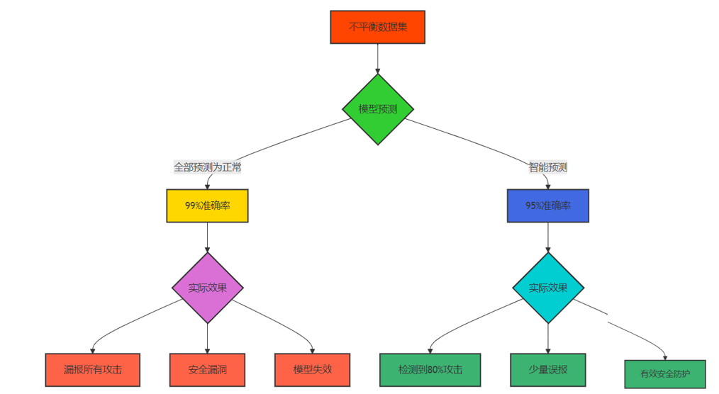
Accuracy = (True Positive + True Negative) / (True Positive + True Negative + False Positive + False Negative)

import numpy as np
import pandas as pd
from sklearn.dummy import DummyClassifier
from sklearn.ensemble import RandomForestClassifier
from sklearn.model_selection import train_test_split
from sklearn.metrics import accuracy_score, precision_score, recall_score, f1_score
from sklearn.datasets import make_classification

# 生成极端不平衡的安全数据集（99%正常，1%攻击）
X, y = make_classification(
    n_samples=10000,
    n_classes=2,
    weights=[0.99, 0.01],
    random_state=42
)

# 划分训练集和测试集
X_train, X_test, y_train, y_test = train_test_split(
    X, y, test_size=0.2, random_state=42, stratify=y
)

print(f"训练集样本数: {len(X_train)}, 攻击样本数: {np.sum(y_train)}")
print(f"测试集样本数: {len(X_test)}, 攻击样本数: {np.sum(y_test)}")
print(f"测试集攻击样本比例: {np.sum(y_test)/len(y_test):.2%}")

# 1. 基准模型：总是预测为正常样本
dummy_model = DummyClassifier(strategy="most_frequent", random_state=42)
dummy_model.fit(X_train, y_train)
dummy_pred = dummy_model.predict(X_test)

# 2. 随机森林模型：智能预测
rf_model = RandomForestClassifier(
    n_estimators=100,
    max_depth=10,
    class_weight="balanced",
    random_state=42
)
rf_model.fit(X_train, y_train)
rf_pred = rf_model.predict(X_test)

# 3. 计算各种评估指标
def calculate_metrics(y_true, y_pred, model_name):
    accuracy = accuracy_score(y_true, y_pred)
    precision = precision_score(y_true, y_pred)
    recall = recall_score(y_true, y_pred)
    f1 = f1_score(y_true, y_pred)
    
    print(f"\n{model_name} 指标:")
    print(f"准确率: {accuracy:.4f}")
    print(f"精确率: {precision:.4f}")
    print(f"召回率: {recall:.4f}")
    print(f"F1分数: {f1:.4f}")
    
    return {
        "模型名称": model_name,
        "准确率": accuracy,
        "精确率": precision,
        "召回率": recall,
        "F1分数": f1
    }

# 计算并比较两个模型的指标
metrics = []
metrics.append(calculate_metrics(y_test, dummy_pred, "总是预测为正常"))
metrics.append(calculate_metrics(y_test, rf_pred, "随机森林模型"))

# 转换为DataFrame进行比较
metrics_df = pd.DataFrame(metrics)
print("\n=== 模型指标对比 ===")
print(metrics_df)

# 计算漏报的攻击样本数
dummy_missed_attacks = np.sum(y_test) - np.sum((dummy_pred == 1) & (y_test == 1))
rf_missed_attacks = np.sum(y_test) - np.sum((rf_pred == 1) & (y_test == 1))

print(f"\n=== 漏报情况分析 ===")
print(f"测试集中攻击样本总数: {np.sum(y_test)}")
print(f"总是预测为正常模型漏报攻击样本数: {dummy_missed_attacks}")
print(f"随机森林模型漏报攻击样本数: {rf_missed_attacks}")
print(f"随机森林模型检测到的攻击样本数: {np.sum(y_test) - rf_missed_attacks}")

import numpy as np
import matplotlib.pyplot as plt
from sklearn.datasets import make_classification
from sklearn.model_selection import train_test_split
from sklearn.ensemble import RandomForestClassifier
from sklearn.metrics import (
    accuracy_score, precision_score, recall_score, f1_score,
    roc_auc_score, average_precision_score, precision_recall_curve, roc_curve
)

# 生成不同不平衡程度的安全数据集
def generate_imbalanced_data(imbalance_ratio):
    return make_classification(
        n_samples=10000,
        n_classes=2,
        weights=[imbalance_ratio, 1 - imbalance_ratio],
        random_state=42
    )

# 测试不同不平衡程度下的指标表现
imbalance_ratios = [0.99, 0.95, 0.9, 0.8, 0.7, 0.5]  # 从极端不平衡到平衡
results = []

for ratio in imbalance_ratios:
    # 生成数据
    X, y = generate_imbalanced_data(ratio)
    
    # 划分训练集和测试集
    X_train, X_test, y_train, y_test = train_test_split(
        X, y, test_size=0.2, random_state=42, stratify=y
    )
    
    # 训练随机森林模型
    model = RandomForestClassifier(
        n_estimators=100,
        max_depth=10,
        class_weight="balanced",
        random_state=42
    )
    model.fit(X_train, y_train)
    
    # 预测
    y_pred = model.predict(X_test)
    y_pred_proba = model.predict_proba(X_test)[:, 1]
    
    # 计算指标
    accuracy = accuracy_score(y_test, y_pred)
    precision = precision_score(y_test, y_pred)
    recall = recall_score(y_test, y_pred)
    f1 = f1_score(y_test, y_pred)
    roc_auc = roc_auc_score(y_test, y_pred_proba)
    pr_auc = average_precision_score(y_test, y_pred_proba)
    
    # 记录结果
    results.append({
        "不平衡比例": ratio,
        "攻击样本比例": 1 - ratio,
        "准确率": accuracy,
        "精确率": precision,
        "召回率": recall,
        "F1分数": f1,
        "ROC-AUC": roc_auc,
        "PR-AUC": pr_auc
    })

# 转换为DataFrame进行分析
import pandas as pd
results_df = pd.DataFrame(results)
print("=== 不同不平衡程度下的指标表现 ===")
print(results_df.round(4))

# 可视化不同指标随不平衡程度的变化
plt.figure(figsize=(12, 8))

# 准确率 vs 其他指标
plt.subplot(2, 2, 1)
plt.plot(results_df["攻击样本比例"], results_df["准确率"], label="准确率", marker="o")
plt.plot(results_df["攻击样本比例"], results_df["F1分数"], label="F1分数", marker="s")
plt.xlabel("攻击样本比例")
plt.ylabel("分数")
plt.title("准确率 vs F1分数")
plt.legend()
plt.grid(True)

# 精确率 vs 召回率
plt.subplot(2, 2, 2)
plt.plot(results_df["攻击样本比例"], results_df["精确率"], label="精确率", marker="o")
plt.plot(results_df["攻击样本比例"], results_df["召回率"], label="召回率", marker="s")
plt.xlabel("攻击样本比例")
plt.ylabel("分数")
plt.title("精确率 vs 召回率")
plt.legend()
plt.grid(True)

# ROC-AUC vs PR-AUC
plt.subplot(2, 2, 3)
plt.plot(results_df["攻击样本比例"], results_df["ROC-AUC"], label="ROC-AUC", marker="o")
plt.plot(results_df["攻击样本比例"], results_df["PR-AUC"], label="PR-AUC", marker="s")
plt.xlabel("攻击样本比例")
plt.ylabel("分数")
plt.title("ROC-AUC vs PR-AUC")
plt.legend()
plt.grid(True)

plt.tight_layout()
plt.savefig("metrics_comparison.png")
print("\n指标对比可视化完成，保存为metrics_comparison.png")

# 分析准确率的误导性
print("\n=== 准确率误导性分析 ===")
print("当攻击样本比例为1%时:")
print(f"- 准确率: {results_df.loc[0, '准确率']:.4f} (看起来很好)")
print(f"- F1分数: {results_df.loc[0, 'F1分数']:.4f} (实际效果较差)")
print(f"- PR-AUC: {results_df.loc[0, 'PR-AUC']:.4f} (更真实地反映模型性能)")

print("\n当攻击样本比例为50%时:")
print(f"- 准确率: {results_df.loc[5, '准确率']:.4f}")
print(f"- F1分数: {results_df.loc[5, 'F1分数']:.4f}")
print(f"- PR-AUC: {results_df.loc[5, 'PR-AUC']:.4f}")
print("\n结论: 随着数据集不平衡程度增加，准确率越来越具有误导性，而PR-AUC和F1分数能更真实地反映模型性能。")

import numpy as np
import pandas as pd
from sklearn.datasets import make_classification
from sklearn.model_selection import train_test_split
from sklearn.ensemble import RandomForestClassifier
from sklearn.metrics import (
    accuracy_score, precision_score, recall_score, f1_score,
    roc_auc_score, average_precision_score, fbeta_score
)

# 生成安全数据集
X, y = make_classification(
    n_samples=10000,
    n_classes=2,
    weights=[0.95, 0.05],
    random_state=42
)

X_train, X_test, y_train, y_test = train_test_split(
    X, y, test_size=0.2, random_state=42, stratify=y
)

# 训练不同参数的随机森林模型
models = {
    "默认参数": RandomForestClassifier(random_state=42),
    "平衡权重": RandomForestClassifier(class_weight="balanced", random_state=42),
    "深度限制": RandomForestClassifier(max_depth=8, class_weight="balanced", random_state=42),
    "更多树": RandomForestClassifier(n_estimators=200, class_weight="balanced", random_state=42)
}

# 训练模型并预测
predictions = {}
for name, model in models.items():
    model.fit(X_train, y_train)
    y_pred = model.predict(X_test)
    y_pred_proba = model.predict_proba(X_test)[:, 1]
    predictions[name] = (y_pred, y_pred_proba)

# 定义不同安全场景的误判成本
scenarios = {
    "入侵检测": {
        "场景描述": "漏报攻击可能导致系统被入侵，成本高；误报正常流量影响较小",
        "beta": 2.0,  # 更看重召回率
        "假阴性成本": 100,  # 漏报1次攻击的成本
        "假阳性成本": 1     # 误报1次正常流量的成本
    },
    "反垃圾邮件": {
        "场景描述": "误报正常邮件可能导致重要信息丢失，成本高；漏报垃圾邮件影响较小",
        "beta": 0.5,  # 更看重精确率
        "假阴性成本": 1,     # 漏报1封垃圾邮件的成本
        "假阳性成本": 50     # 误报1封正常邮件的成本
    },
    "欺诈检测": {
        "场景描述": "漏报欺诈交易导致直接经济损失；误报正常交易影响用户体验",
        "beta": 1.5,  # 稍微看重召回率
        "假阴性成本": 1000,  # 漏报1次欺诈的成本
        "假阳性成本": 10     # 误报1次正常交易的成本
    }
}

# 计算不同场景下的最佳模型
def calculate_scenario_metrics(y_true, y_pred, y_pred_proba, scenario):
    # 基本指标
    accuracy = accuracy_score(y_true, y_pred)
    precision = precision_score(y_true, y_pred)
    recall = recall_score(y_true, y_pred)
    f1 = f1_score(y_true, y_pred)
    
    # 场景特定指标
    fbeta = fbeta_score(y_true, y_pred, beta=scenario["beta"])
    roc_auc = roc_auc_score(y_true, y_pred_proba)
    pr_auc = average_precision_score(y_true, y_pred_proba)
    
    # 计算总成本
    tn, fp, fn, tp = np.bincount(y_true.astype(int) * 2 + y_pred.astype(int), minlength=4)
    total_cost = fn * scenario["假阴性成本"] + fp * scenario["假阳性成本"]
    
    return {
        "准确率": accuracy,
        "精确率": precision,
        "召回率": recall,
        "F1分数": f1,
        "F-beta分数": fbeta,
        "ROC-AUC": roc_auc,
        "PR-AUC": pr_auc,
        "总成本": total_cost
    }

# 分析不同场景下的模型表现
for scenario_name, scenario in scenarios.items():
    print(f"\n=== {scenario_name} 场景分析 ===")
    print(f"场景描述: {scenario['场景描述']}")
    print(f"F-beta的beta值: {scenario['beta']}")
    
    scenario_results = []
    for model_name, (y_pred, y_pred_proba) in predictions.items():
        metrics = calculate_scenario_metrics(y_test, y_pred, y_pred_proba, scenario)
        metrics["模型名称"] = model_name
        scenario_results.append(metrics)
    
    # 转换为DataFrame并排序
    df = pd.DataFrame(scenario_results)
    df = df.sort_values(by="总成本")
    
    print(f"\n{scenario_name}场景下模型表现（按总成本排序）:")
    print(df.round(4))
    
    # 找出最佳模型
    best_model = df.iloc[0]
    print(f"\n{scenario_name}场景下的最佳模型: {best_model['模型名称']}")
    print(f"- 准确率: {best_model['准确率']:.4f}")
    print(f"- F-beta分数: {best_model['F-beta分数']:.4f}")
    print(f"- PR-AUC: {best_model['PR-AUC']:.4f}")
    print(f"- 总成本: {best_model['总成本']}")
    
    # 比较准确率和总成本
    accuracy_based = df.sort_values(by="准确率", ascending=False).iloc[0]
    print(f"\n如果仅基于准确率选择模型: {accuracy_based['模型名称']}")
    print(f"- 准确率: {accuracy_based['准确率']:.4f}")
    print(f"- 总成本: {accuracy_based['总成本']}")
    print(f"- 成本差异: {accuracy_based['总成本'] - best_model['总成本']}")

print("\n=== 结论 ===")
print("1. 不同安全场景需要选择不同的评估指标")
print("2. 仅基于准确率选择模型可能导致成本大幅增加")
print("3. 考虑误判成本的F-beta分数和总成本是更合理的选择")
print("4. PR-AUC比ROC-AUC更适合不平衡的安全数据集")

import numpy as np
from sklearn.metrics import (
    accuracy_score, precision_score, recall_score, f1_score,
    fbeta_score, roc_auc_score, average_precision_score,
    confusion_matrix
)

def compute_all_metrics(y_true, y_pred, y_pred_proba=None, beta=1.0):
    """计算安全场景下的所有常用评估指标"""
    
    # 基本指标
    accuracy = accuracy_score(y_true, y_pred)
    precision = precision_score(y_true, y_pred)
    recall = recall_score(y_true, y_pred)
    f1 = f1_score(y_true, y_pred)
    fbeta = fbeta_score(y_true, y_pred, beta=beta)
    
    # 混淆矩阵
    tn, fp, fn, tp = confusion_matrix(y_true, y_pred).ravel()
    
    # 衍生指标
    fpr = fp / (fp + tn)  # 假阳性率
    fnr = fn / (fn + tp)  # 假阴性率
    tpr = tp / (tp + fn)  # 真阳性率（召回率）
    tnr = tn / (tn + fp)  # 真阴性率
    
    # 概率相关指标
    roc_auc = None
    pr_auc = None
    if y_pred_proba is not None:
        roc_auc = roc_auc_score(y_true, y_pred_proba)
        pr_auc = average_precision_score(y_true, y_pred_proba)
    
    return {
        "accuracy": accuracy,
        "precision": precision,
        "recall": recall,
        "f1": f1,
        "fbeta": fbeta,
        "roc_auc": roc_auc,
        "pr_auc": pr_auc,
        "fpr": fpr,
        "fnr": fnr,
        "tpr": tpr,
        "tnr": tnr,
        "confusion_matrix": {
            "tp": tp,
            "fp": fp,
            "fn": fn,
            "tn": tn
        }
    }

def calculate_cost(y_true, y_pred, false_negative_cost, false_positive_cost):
    """计算模型的总成本"""
    tn, fp, fn, tp = confusion_matrix(y_true, y_pred).ravel()
    total_cost = fn * false_negative_cost + fp * false_positive_cost
    return total_cost

def print_metrics(metrics, name="模型"):
    """打印评估指标"""
    print(f"\n=== {name} 评估指标 ===")
    print(f"准确率: {metrics['accuracy']:.4f}")
    print(f"精确率: {metrics['precision']:.4f}")
    print(f"召回率: {metrics['recall']:.4f}")
    print(f"F1分数: {metrics['f1']:.4f}")
    print(f"F-beta分数: {metrics['fbeta']:.4f}")
    print(f"假阳性率: {metrics['fpr']:.4f}")
    print(f"假阴性率: {metrics['fnr']:.4f}")
    
    if metrics['roc_auc'] is not None:
        print(f"ROC-AUC: {metrics['roc_auc']:.4f}")
    if metrics['pr_auc'] is not None:
        print(f"PR-AUC: {metrics['pr_auc']:.4f}")
    
    cm = metrics['confusion_matrix']
    print(f"\n混淆矩阵:")
    print(f"  预测正常 | 预测攻击")
    print(f"实际正常 | {cm['tn']:8d} | {cm['fp']:8d}")
    print(f"实际攻击 | {cm['fn']:8d} | {cm['tp']:8d}")