pygrib | 读取CFS数据及简单可视化

用户11172986

发布于 2025-03-06 23:28:38

1300

代码可运行

文章被收录于专栏：气python风雨气python风雨

运行总次数：0

代码可运行

pygrib | 读取CFS数据及简单可视化

前言

之前在评论区有朋友留言想看pygrib的安装教程，我测试了一下。

结果在上期的虚拟环境下直接使用pip install 啪的一下装好了

你小子谎报军情是吧，哪里有什么难度（恼）

既然来都来了还是扩展一下写写CFS的数据处理

本文适合读者

气象数据分析师
Python数据处理爱好者
气候研究科研人员

🌦️ 为什么要处理GRIB数据？

GRIB（GRIdded Binary）格式是气象领域最常用的数据格式之一，具有：

高效压缩：适合存储大规模气象要素场
多维支持：可包含时间、高度层、预报时效等多个维度
元数据丰富：包含要素单位、坐标参考系等重要信息

CFS（气候预报系统）产生的预报数据大多采用GRIB2格式存储，掌握其处理技能是气象数据分析的基本功。

🛠️ 准备工作

1. 安装核心库

pip install pygrib matplotlib cartopy

📖 代码实战

1. 读取GRIB数据

import pygrib

# 打开GRIB文件
grbs = pygrib.open('/home/mw/input/cfs85518551/flxf2025070818.01.2025022700.grb2')

# 列出所有数据层
for grb in grbs[1:20]:
    print(grb)

1:Momentum flux, u component:N m**-2 (instant):regular_gg:surface:level 0:fcst time 3162 hrs:from 202502270000
2:Momentum flux, v component:N m**-2 (instant):regular_gg:surface:level 0:fcst time 3162 hrs:from 202502270000
3:Instantaneous surface sensible heat flux:W m**-2 (instant):regular_gg:surface:level 0:fcst time 3162 hrs:from 202502270000
4:Latent heat net flux:W m**-2 (instant):regular_gg:surface:level 0:fcst time 3162 hrs:from 202502270000
5:Temperature:K (instant):regular_gg:surface:level 0:fcst time 3162 hrs:from 202502270000
6:Volumetric soil moisture content:Proportion (instant):regular_gg:depthBelowLandLayer:levels 0.0-0.1 m:fcst time 3162 hrs:from 202502270000
7:Volumetric soil moisture content:Proportion (instant):regular_gg:depthBelowLandLayer:levels 0.1-0.4 m:fcst time 3162 hrs:from 202502270000
8:Temperature:K (instant):regular_gg:depthBelowLandLayer:levels 0.0-0.1 m:fcst time 3162 hrs:from 202502270000
9:Temperature:K (instant):regular_gg:depthBelowLandLayer:levels 0.1-0.4 m:fcst time 3162 hrs:from 202502270000
10:Water equivalent of accumulated snow depth (deprecated):kg m**-2 (instant):regular_gg:surface:level 0:fcst time 3162 hrs:from 202502270000
11:Downward long-wave radiation flux:W m**-2 (instant):regular_gg:surface:level 0:fcst time 3162 hrs:from 202502270000
12:Upward long-wave radiation flux:W m**-2 (instant):regular_gg:surface:level 0:fcst time 3162 hrs:from 202502270000
13:Upward long-wave radiation flux:W m**-2 (instant):regular_gg:nominalTop:level 0:fcst time 3162 hrs:from 202502270000
14:Upward short-wave radiation flux:W m**-2 (instant):regular_gg:nominalTop:level 0:fcst time 3162 hrs:from 202502270000
15:Upward short-wave radiation flux:W m**-2 (instant):regular_gg:surface:level 0:fcst time 3162 hrs:from 202502270000
16:Downward short-wave radiation flux:W m**-2 (instant):regular_gg:surface:level 0:fcst time 3162 hrs:from 202502270000
17:UV-B downward solar flux:W m**-2 (instant):regular_gg:surface:level 0:fcst time 3162 hrs:from 202502270000
18:Clear sky UV-B downward solar flux:W m**-2 (instant):regular_gg:surface:level 0:fcst time 3162 hrs:from 202502270000
19:Total Cloud Cover:% (instant):regular_gg:highCloudLayer:level 0:fcst time 3162 hrs:from 202502270000

2. 获取u变量与经纬度

grb = grbs.select(name='Momentum flux, u component', forecastTime=3162)[0]
U    = grb.values
lat, lon = grb.latlons()

# 关闭文件
grbs.close()

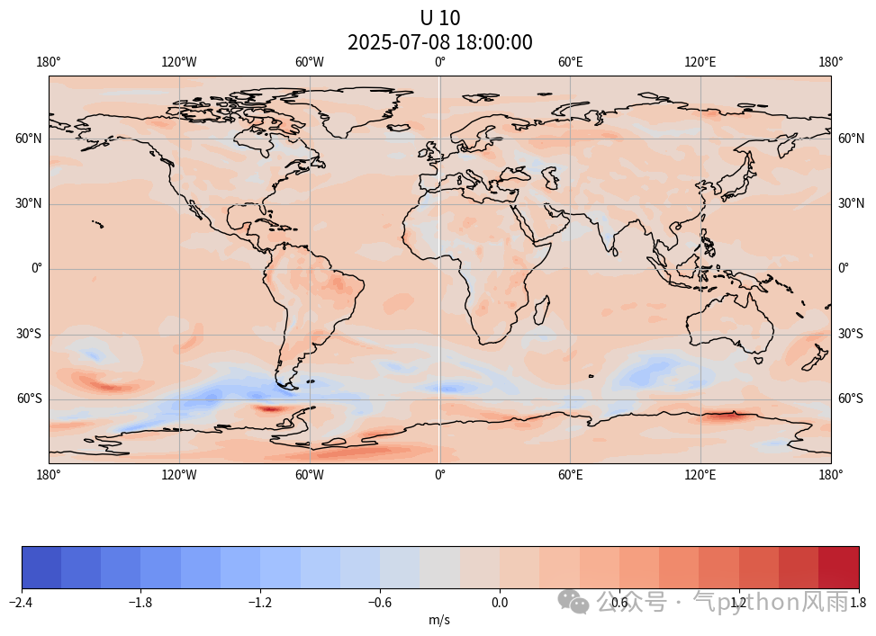
3. 数据可视化


import matplotlib.pyplot as plt
import cartopy.crs as ccrs
import cartopy.feature as cfeature

# 创建画布
fig = plt.figure(figsize=(12, 8))
ax = fig.add_subplot(111, projection=ccrs.PlateCarree())

# 绘制填色图
contour = ax.contourf(lon, lat, U, 
                     transform=ccrs.PlateCarree(),
                     cmap='coolwarm',
                     levels=20)

# 添加地理要素
ax.add_feature(cfeature.COASTLINE)
ax.gridlines(draw_labels=True)

# 添加色标
plt.colorbar(contour, orientation='horizontal', 
            label='m/s')

# 设置标题
plt.title(f'U 10\n{grb.validDate}', size=16)

plt.savefig('cfs_u10.png', dpi=300, bbox_inches='tight')

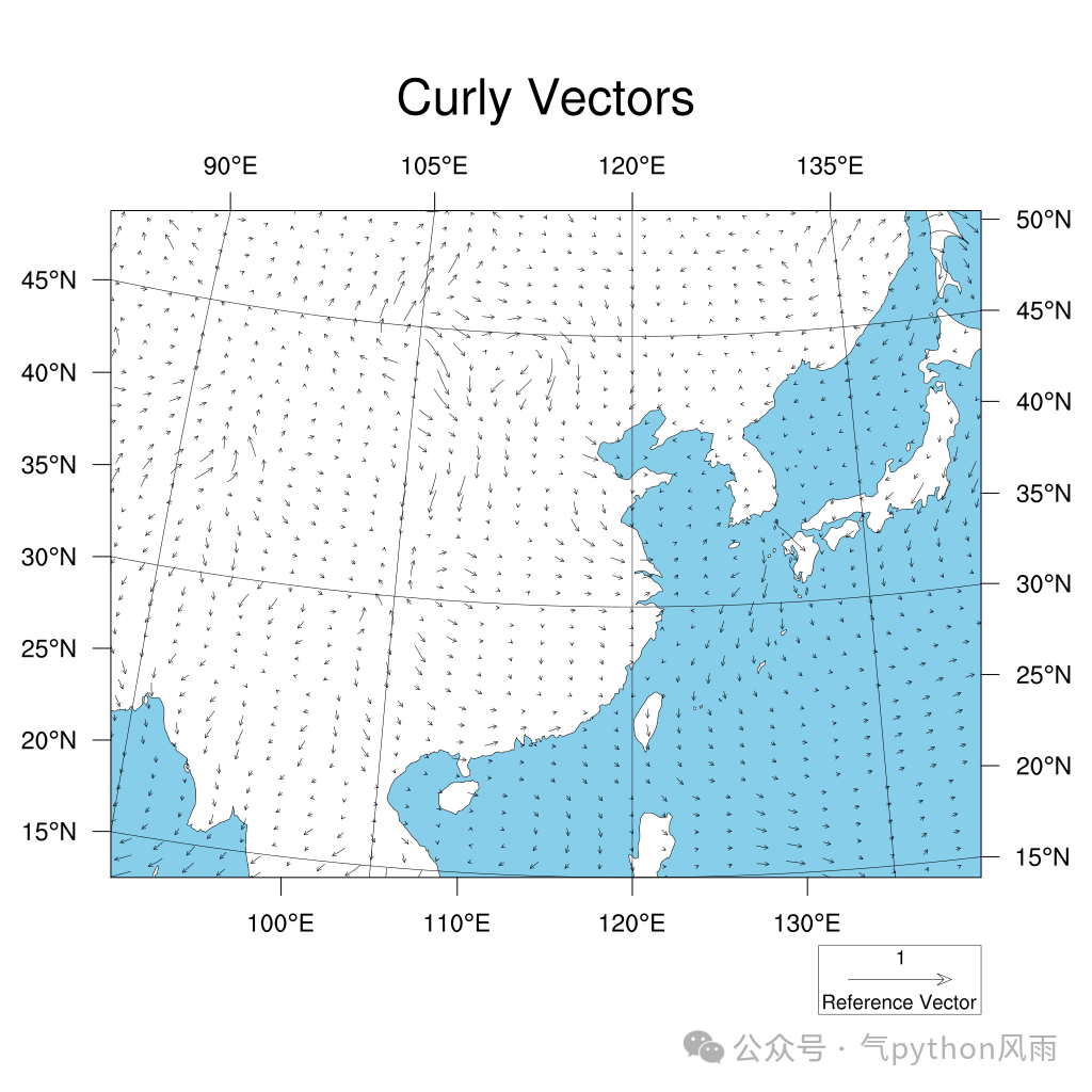
4. 细化绘图

import pygrib

# 打开GRIB文件
grbs = pygrib.open('/home/mw/input/cfs85518551/flxf2025070818.01.2025022700.grb2')

grb_u = grbs.select(name='Momentum flux, u component')[0]
grb_v = grbs.select(name='Momentum flux, v component')[0]

# 提取U和V的值
u = grb_u.values
v = grb_v.values

# 提取经纬度
lat, lon = grb_u.latlons()

# 关闭文件
grbs.close()