新秀mulea包能取代y叔的clusterProfiler包生物学功能富集分析吗？

生信技能树

发布于 2024-12-19 18:33:30

11400

代码可运行

文章被收录于专栏：生信技能树生信技能树

运行总次数：0

代码可运行

mulea R 包是一个全面的功能性富集分析工具，它提供了两种不同的方法：

对于非排序元素，如显著上、下调基因，mulea 采用基于集合的过表达分析（overrepresentation analysis 、ORA）。mulea 采用了一种渐进的经验假发现率（eFDR）方法，这种方法专门为相互关联的生物数据设计，以准确识别不同GO中的显著Term。
对于排序元素，例如按 p 值或差异表达分析计算的 log2FC 排序的基因，mulea 提供基因集富集（GSEA）方法。

mulea 超越了传统工具，通过整合广泛的本体论，包括基因本体论、通路、调控元件、基因组位置和蛋白质域，涵盖27个模型生物，覆盖来自16个数据库的22种本体论类型和各种标识符，结果在 ELTEbioinformatics/GMT_files_for_mulea GitHub 存储库和通过 muleaData ExperimentData Bioconductor 包中有879个文件可用。

网址：https://github.com/ELTEbioinformatics/mulea

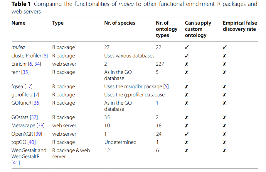
功能富集分析包比较一览：

支持27个模式物种：

安装此包：

# 设置镜像：
options(BioC_mirror="https://mirrors.westlake.edu.cn/bioconductor")
options("repos"=c(CRAN="https://mirrors.westlake.edu.cn/CRAN/"))

# 安装依赖：
# Installing the fgsea package with the BiocManager
BiocManager::install("fgsea")


# Installing the devtools package if needed
if (!require("devtools", quietly = TRUE))
    install.packages("devtools")

# Installing the mulea package from GitHub
devtools::install_github("https://github.com/ELTEbioinformatics/mulea")

小试牛刀

加载R包

library(mulea)
library(tidyverse)

一、加载基因集

这部分展示如果导入各种资源的基因集，例如从Regulon数据库下载的转录因子及其靶基因，并确保研究元素之间的标识符类型（例如，UniProt蛋白质ID、Entrez ID、基因符号、Ensembl基因ID）相匹配。

方法1：从gmt格式导入

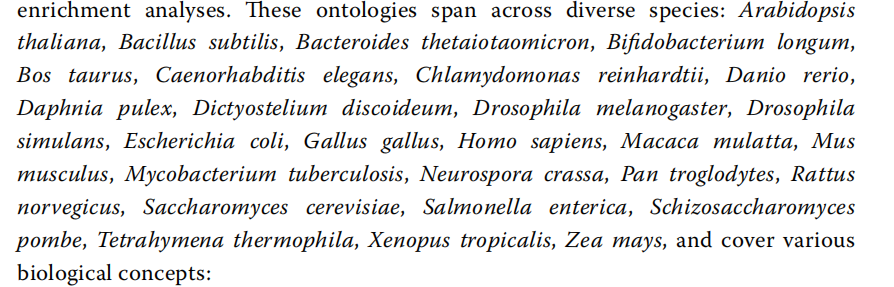
gmt为tab键分割，一行为一个基因集，可以使用mule包中的 read_gmt 函数进行读取，这个包中 https://github.com/ELTEbioinformatics/GMT_files_for_mulea 提供了27个物种，16个公开数据库的gmt格式文件。

物种列表：

我们涵盖的物种列表：拟南芥 (Arabidopsis thaliana) 枯草杆菌 (Bacillus subtilis) 嗜粘蛋白-梭菌 (Bacteroides thetaiotaomicron VPI-5482) 长双歧杆菌 (Bifidobacterium longum) 牛 (Bos taurus) 秀丽隐杆线虫 (Caenorhabditis elegans) 莱茵衣藻 (Chlamydomonas reinhardtii) 斑马鱼 (Danio rerio) 水蚤 (Daphnia pulex) 黏菌 (Dictyostelium discoideum) 果蝇 (Drosophila melanogaster) 拟果蝇 (Drosophila simulans) 大肠杆菌 (Escherichia coli) 鸡 (Gallus gallus) 人类 (Homo sapiens) 猕猴 (Macaca mulatta) 小鼠 (Mus musculus) 结核分枝杆菌 (Mycobacterium tuberculosis) 粗糙链孢霉 (Neurospora crassa) 黑猩猩 (Pan troglodytes) 大鼠 (Rattus norvegicus) 酿酒酵母 (Saccharomyces cerevisiae) 鼠伤寒沙门氏菌 (Salmonella enterica subsp. enterica serovar Typhimurium str. LT2) 裂殖酵母 (Schizosaccharomyces pombe) 嗜热四膜虫 (Tetrahymena thermophila) 热带爪蟾 (Xenopus tropicalis) 玉米 (Zea mays)

直接从github上读取：

# Reading the GMT file from the GitHub repository
tf_ontology <- read_gmt("https://raw.githubusercontent.com/ELTEbioinformatics/GMT_files_for_mulea/main/GMT_files/Escherichia_coli_83333/Transcription_factor_RegulonDB_Escherichia_coli_GeneSymbol.gmt")

class(tf_ontology)
head(tf_ontology)

或者下载到本地再读取：

# Reading the mulea GMT file locally
tf_ontology <- read_gmt("Transcription_factor_RegulonDB_Escherichia_coli_GeneSymbol.gmt")

还有另外一种GMT File来自Enricher R包：

# Reading the Enrichr GMT file locally
tf_enrichr_ontology <- read_gmt("TRRUST_Transcription_Factors_2019.txt")

# The ontology_name is empty, therefore we need to fill it with the ontology_id
tf_enrichr_ontology$ontology_name <- tf_enrichr_ontology$ontology_id

还有来自大家都知道的 MsigDB 数据库的GMT File：

# 需要从官网下载下来，默认大家都会从msigdb数据库去下载gmt基因集
# Reading the MsigDB GMT file locally
tf_msigdb_ontology <- read_gmt("c3.tft.v2023.2.Hs.symbols.gmt")

方法2：使用`muleaData`内置的基因集

# Installing the ExperimentHub package from Bioconductor
# BiocManager::install("ExperimentHub")
# Calling the ExperimentHub library.
library(ExperimentHub)
# Downloading the metadata from ExperimentHub.
eh <- ExperimentHub()

# Creating the muleaData variable.
muleaData <- query(eh, "muleaData")

# Looking for the ExperimentalHub ID of the ontology.
EHID <- mcols(muleaData) %>% 
  as.data.frame() %>% 
  dplyr::filter(title == "Transcription_factor_RegulonDB_Escherichia_coli_GeneSymbol.rds") %>% 
  rownames()

# Reading the ontology from the muleaData package.
tf_ontology <- muleaData[[EHID]]

# Change the header
tf_ontology <- tf_ontology %>% 
  rename(ontology_id = "ontologyId",
         ontology_name = "ontologyName",
         list_of_values = "listOfValues")

过滤基因集

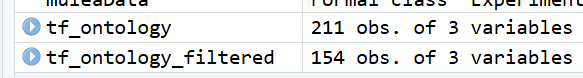
富集分析的结果有时会因为过于具体或广泛的条目而产生偏差。mulea 允许自定义go term的大小——即属于一个术语的基因或蛋白质的数量——确保你的分析符合你期望的范围。

让我们排除基因少于3个或多于400个的go term：

# Filtering the ontology
tf_ontology_filtered <- filter_ontology(gmt = tf_ontology,
                                        min_nr_of_elements = 3,
                                        max_nr_of_elements = 400)

过滤前后：

保存

使用 **write_gmt**函数保存gmt数据：

# Saving the ontology to GMT file
write_gmt(gmt = tf_ontology_filtered, file = "Filtered.gmt")

list对象转换为 Ontology Object对象

mulea 包提供了 list_to_gmt 函数，用于将基因集列表转换为本体论数据框架。以下示例展示了如何使用这个函数：

# Creating a list of gene sets
ontology_list <- list(gene_set1 = c("gene1", "gene2", "gene3"),
                      gene_set2 = c("gene4", "gene5", "gene6"))

# Converting the list to a ontology (GMT) object
new_ontology_df <- list_to_gmt(ontology_list)

示例数据

数据来自GEO：https://www.ncbi.nlm.nih.gov/geo/query/acc.cgi?acc=GSE55662

次数据的研究调查了大肠杆菌中抗生素抗性进化的情况。比较了环丙沙星ciprofloxacin抗生素处理的大肠杆菌与未处理对照组之间的基因表达变化。使用GEO2R工具比较了这些组的表达水平：

未处理对照样本（2个重复）：WT_noCPR_1, WT_noCPR_2
环丙沙星处理样本（2个重复）：WT_CPR_1, WT_CPR_2

二、对于非排序元素：Overrepresentation Analysis (ORA) 分析

mulea 包使用超几何方法进行富集分析，通过 ora 函数实现，需要三个输入数据：

Ontology data frame：即前面取得的各种gmt格式的基因集合
感兴趣基因列表：一个要研究的元素向量，包含感兴趣的基因或蛋白质，例如实验中显著过表达的基因。
背景基因集：一般为所有检测的基因或者蛋白

# Taget set 感兴趣基因列表
target_set <- readLines("mulea-master/inst/extdata/target_set.txt")
target_set
head(target_set)
# [1] "gnsB"  "sulA"  "recN"  "c4435" "dinI"  "c2757"
length(target_set)
# [1] 241


# 背景基因集
background_set <- readLines("mulea-master/inst/extdata/background_set.txt")
background_set
length(background_set)
# [1] 7381

执行 OverRepresentation Analysis

运行 10,000 permutations 计算 eFDR

# Creating the ORA model using the GMT variable
ora_model <- ora(gmt = tf_ontology_filtered, 
                 # Test set variable
                 element_names = target_set, 
                 # Background set variable
                 background_element_names = background_set, 
                 # p-value adjustment method
                 p_value_adjustment_method = "eFDR", 
                 # Number of permutations
                 number_of_permutations = 10000,
                 # Number of processor threads to use
                 nthreads = 2, 
                 # Setting a random seed for reproducibility
                 random_seed = 1) 

# Running the ORA
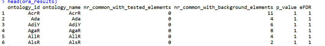
ora_results <- run_test(ora_model)
head(ora_results)

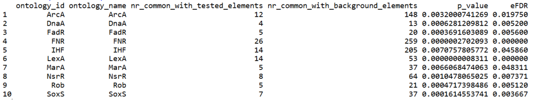
得到的结果如下：

挑选显著ORA结果

ora_results %>%
  # Rows where the eFDR < 0.05
  filter(eFDR < 0.05) %>% 
  # Number of such rows
  nrow()
#> [1] 10

ora_results %>%
  # Arrange the rows by the eFDR values
  arrange(eFDR) %>% 
  # Rows where the eFDR < 0.05
  filter(eFDR < 0.05)

10条term efdr<0.05

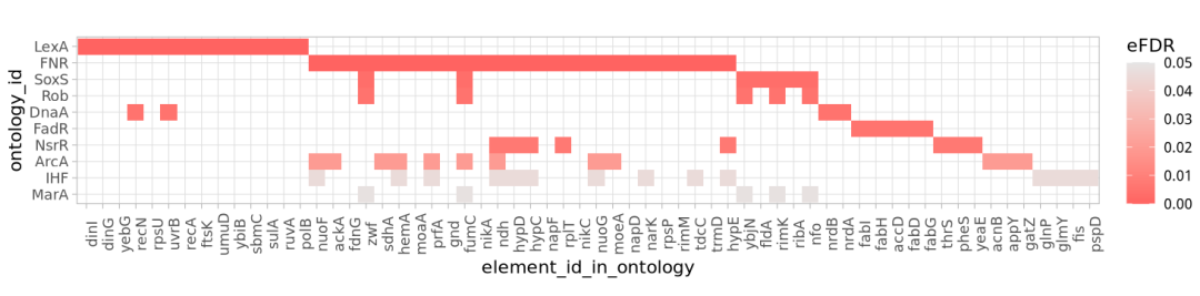
可视化

mulea 提供了多种可视化工具，包括棒棒糖图、条形图、网络图和热图。这些可视化有效地揭示了富集因子之间的模式和关系。

使用 reshape_results 函数初始化可视化：

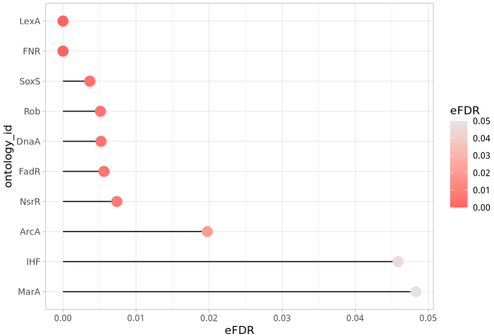
可视化eFDR值的分布：棒棒糖图

棒棒糖图提供了富集转录因子分布的图形表示。y轴显示转录因子，而x轴代表它们对应的eFDR值。点的颜色根据它们的eFDR值进行着色。这种可视化帮助我们检查eFDR的分布，并识别超过常用的0.05显著性阈值的因子。

plot_lollipop(reshaped_results = ora_reshaped_results,
              # Column containing the names we wish to plot
              ontology_id_colname = "ontology_id",
              # Upper threshold for the value indicating the significance
              p_value_max_threshold = 0.05,
              # Column that indicates the significance values
              p_value_type_colname = "eFDR")

结果如下：

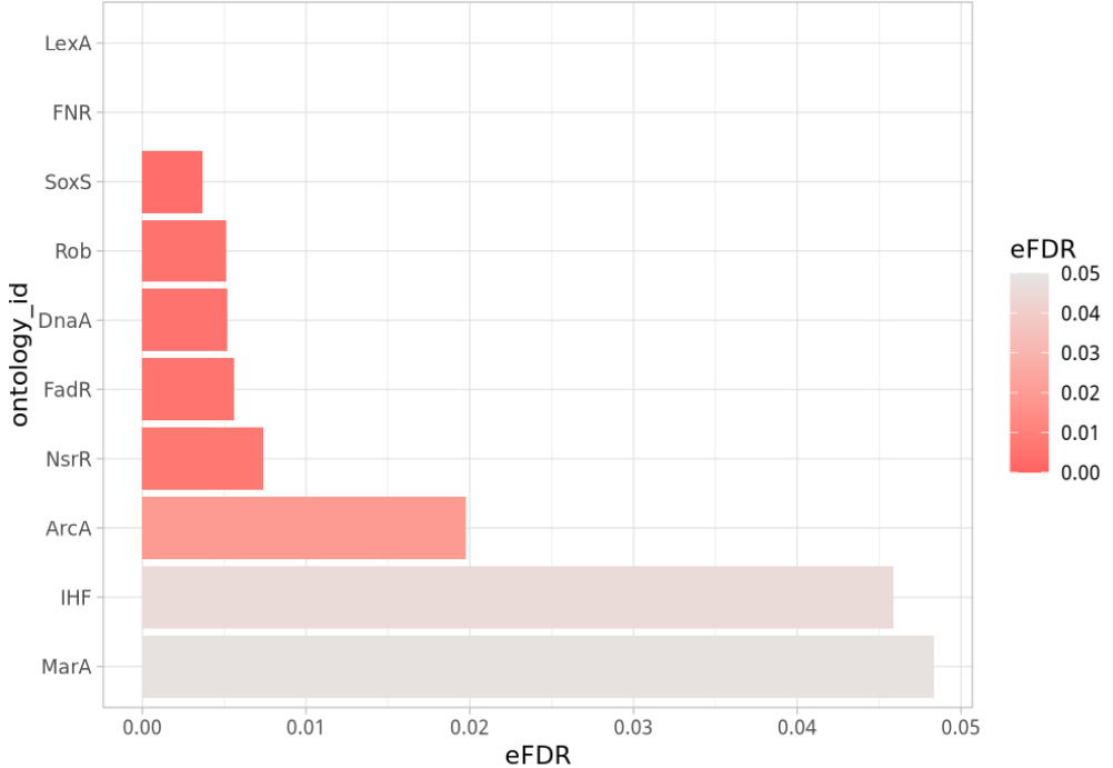
可视化eFDR值的分布：条形图

条形图提供了与棒棒糖图类似的图形表示。y轴显示富集的本体论类别（例如，转录因子），而x轴代表它们对应的eFDR值。条形的颜色根据它们的eFDR值进行着色，这有助于检查eFDR的分布，并识别超过0.05显著性阈值的因子。

plot_barplot(reshaped_results = ora_reshaped_results,
              # Column containing the names we wish to plot
              ontology_id_colname = "ontology_id",
              # Upper threshold for the value indicating the significance
              p_value_max_threshold = 0.05,
              # Column that indicates the significance values
              p_value_type_colname = "eFDR")

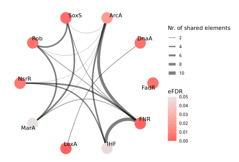
可视化关联：图形图

这个函数生成了一个富集本体论类别（例如，转录因子）的网络可视化。每个节点代表一个富集的本体论类别，根据其eFDR值进行着色。如果两个节点至少共享一个属于目标集合的共同基因，则它们之间会绘制一条边，表示共同调控。边的厚度反映了共享基因的数量。

plot_graph(reshaped_results = ora_reshaped_results,
           # Column containing the names we wish to plot
           ontology_id_colname = "ontology_id",
           # Upper threshold for the value indicating the significance
           p_value_max_threshold = 0.05,
           # Column that indicates the significance values
           p_value_type_colname = "eFDR")

可视化关联：热图

热图显示了与富集本体论类别（例如，转录因子）相关的基因。每一行代表一个类别，根据其eFDR值进行着色。每一列代表一个来自目标集合的基因，该基因属于富集的本体论类别，表明可能受到一个或多个富集转录因子的调控。

plot_heatmap(reshaped_results = ora_reshaped_results,
             # Column containing the names we wish to plot
             ontology_id_colname = "ontology_id",
             # Column that indicates the significance values
             p_value_type_colname = "eFDR")

pvalue矫正：eFDR vs BH vs Bonferroni corrections

ora 函数允许选择不同的方法来计算FDR（假发现率）和调整p值：eFDR，以及stats::p.adjust文档中提供的所有方法选项（holm, hochberg, hommel, bonferroni, BH, BY, 和 fdr）

# Creating the ORA model using the Benjamini-Hochberg p-value correction method
BH_ora_model <- ora(gmt = tf_ontology_filtered, 
                 # Test set variable
                 element_names = target_set, 
                 # Background set variable
                 background_element_names = background_set, 
                 # p-value adjustment method
                 p_value_adjustment_method = "BH") 

# Running the ORA
BH_results <- run_test(BH_ora_model)

# Creating the ORA model using the Bonferroni p-value correction method
Bonferroni_ora_model <- ora(gmt = tf_ontology_filtered, 
                            # Test set variable
                            element_names = target_set, 
                            # Background set variable
                            background_element_names = background_set, 
                            # p-value adjustment method
                            p_value_adjustment_method = "bonferroni") 

# Running the ORA
Bonferroni_results <- run_test(Bonferroni_ora_model)

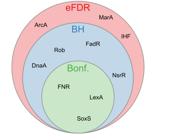
使用阈值cutoff<0.05对三种pvalue矫正方法进行比较：

# Merging the Benjamini-Hochberg and eFDR results
merged_results <- BH_results %>% 
  # Renaming the column
  rename(BH_adjusted_p_value = adjusted_p_value) %>% 
  # Selecting the necessary columns
  select(ontology_id, BH_adjusted_p_value) %>%
  # Joining with the eFDR results
  left_join(ora_results, ., by = "ontology_id") %>% 
  # Converting the data.frame to a tibble
  tibble()

# Merging the Bonferroni results with the merged results
merged_results <- Bonferroni_results %>% 
  # Renaming the column
  rename(Bonferroni_adjusted_p_value = adjusted_p_value) %>% 
  # Selecting the necessary columns
  select(ontology_id, Bonferroni_adjusted_p_value) %>%
  # Joining with the eFDR results
  left_join(merged_results, ., by = "ontology_id") %>% 
  # Arranging by the p-value
  arrange(p_value)

# filter the p-value < 0.05 results
merged_results_filtered <- merged_results %>% 
  filter(p_value < 0.05) %>% 
  # remove the unnecessary columns
  select(-ontology_id, -nr_common_with_tested_elements, 
         -nr_common_with_background_elements)

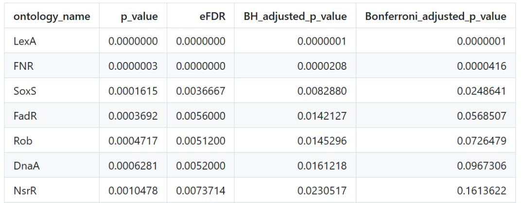
image-20241213012429398

对显著结果的比较显示，传统的p值校正方法（Benjamini-Hochberg和Bonferroni）往往过于保守，导致与eFDR相比，显著转录因子的数量减少。

正如下图所示，通过应用eFDR，我们能够识别出10个显著的转录因子，而使用Benjamini-Hochberg和Bonferroni校正分别只有7个和3个。这表明，在这种情况下，eFDR可能是控制假阳性的更合适的方法。

用后体验：

感觉此方法唯一的亮点是：资源整合，提供了16个数据库的27个物种的gmt 基因集合，而对于里面的ORA和GSEA分析就是前面两个非常经典的做功能富集分析方法的打包，eFDR就是一个置换检验。这个文章发了几分什么杂志我再看一眼啊：

Turek, Cezary, Márton Ölbei, Tamás Stirling, Gergely Fekete, Ervin Tasnádi, Leila Gul, Balázs Bohár, Balázs Papp, Wiktor Jurkowski, and Eszter Ari. 2024. “mulea: An R Package for Enrichment Analysis Using Multiple Ontologies and Empirical False Discovery Rate.” BMC Bioinformatics 25 (1): 334. https://doi.org/10.1186/s12859-024-05948-7.

BMC Bioinformatics的影响因子在2023年为2.9，在Web of Science的分类中，BMC Bioinformatics位于多个学科类别中。在"Biochemical Research Methods"类别下，位于Q3区。在"Biotechnology & Applied Microbiology"类别中，也处于Q3区。在"Mathematical & Computational Biology"类别中，位于Q2区

后面还可以做GSEA分析，大家快去试试看吧！多一个方法不多，可以扩宽见识。

学徒作业

如果大家打开 enrichKEGG {clusterProfiler} 的帮助文档，可以很明显的看到一个案例数据和代码：

library(clusterProfiler)
  data(geneList, package='DOSE')
  de <- names(geneList)[1:100]
  yy <- enrichKEGG(de, pvalueCutoff=0.01)
  head(yy)

这个代码就是加载y叔的成名作clusterProfiler包，然后使用DOSE里面的排序好的基因列表的前100个，然后去做kegg数据库的超几何分布检验。因为kegg数据库版权问题，所以第一次运行这个代码的时候是需要联网下载的：

Reading KEGG annotation online: "https://rest.kegg.jp/link/hsa/pathway"...
Reading KEGG annotation online: "https://rest.kegg.jp/list/pathway/hsa"...

一般来说，问题也不大。给大家一个作业，就是上面的基因列表的前100个，使用我们今天介绍的新秀mulea包试试看做同样的分析，然后对比两次分析的结果！

本文参与腾讯云自媒体同步曝光计划，分享自微信公众号。

原始发表：2024-12-14，如有侵权请联系 cloudcommunity@tencent.com 删除

ontology

本文分享自生信技能树微信公众号，前往查看

如有侵权，请联系 cloudcommunity@tencent.com 删除。

本文参与腾讯云自媒体同步曝光计划，欢迎热爱写作的你一起参与！

登录后参与评论

0 条评论

热度