必看！Seurat赋能 Xenium空间转录组学分析全攻略

天意生信云

发布于 2025-05-12 04:39:17

13100

代码可运行

运行总次数：0

代码可运行

Xenium作为10x Genomics推出的一项先进空间转录组学技术，能够在单细胞分辨率的基础上，精确地检测和定位组织切片中基因的表达情况。通过结合分子检测的灵敏度与空间定位的准确性，Xenium为深入研究细胞在复杂组织环境中的空间位置及其功能和相互关系提供了强大的工具。接下来的内容将以代码为主线，逐步梳理使用Seurat处理和分析此类数据的流程。

官方教程： https://satijalab.org/seurat/articles/seurat5_spatial_vignette_2

数据下载与设置

获取数据：我们使用的是”10x Genomics Xenium小鼠大脑“演示数据集。

wget https://cf.10xgenomics.com/samples/xenium/1.0.2/Xenium_V1_FF_Mouse_Brain_Coronal_Subset_CTX_HP/Xenium_V1_FF_Mouse_Brain_Coronal_Subset_CTX_HP_outs.zip
unzip Xenium_V1_FF_Mouse_Brain_Coronal_Subset_CTX_HP_outs.zip

然后，加载到Seurat中。将 path 指向你的 Xenium_outs 文件夹。

# install.packages("Seurat") # 如果尚未安装
library(Seurat)
# path <- "/你的路径/Xenium_V1_FF_Mouse_Brain_Coronal_Subset_CTX_HP_outs" # 替换为你的实际路径
path <- "Xenium_V1_FF_Mouse_Brain_Coronal_Subset_CTX_HP_outs" # 假设解压在当前目录
xenium.obj <- LoadXenium(path, fov = "fov")
# 移除计数为0的细胞
xenium.obj <- subset(xenium.obj, subset = nCount_Xenium > 0)

这将加载转录本位置、细胞x基因矩阵、细胞分割和细胞质心信息。

初始QC与基因可视化

标准QC图：每个细胞的基因数 (nFeature_Xenium) 和每个细胞的转录本数 (nCount_Xenium)。

VlnPlot(xenium.obj, features = c("nFeature_Xenium", "nCount_Xenium"), ncol = 2, pt.size = 0)

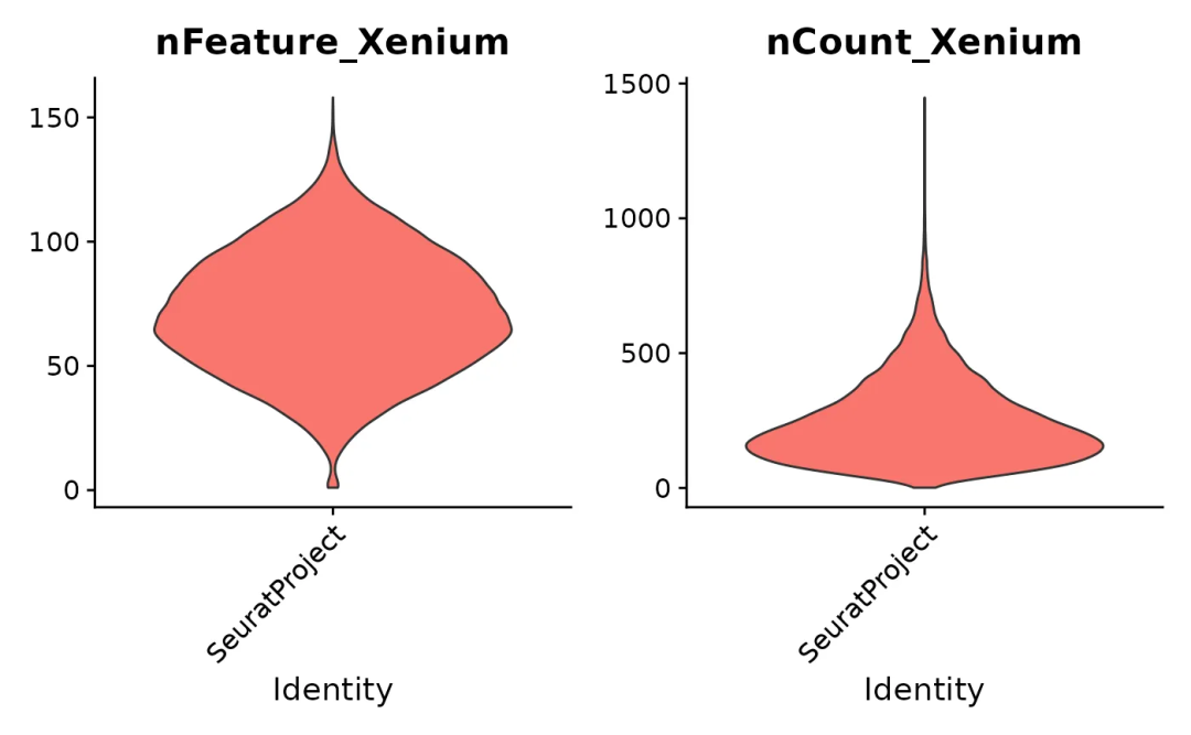
小提琴图显示每个细胞的基因数和转录本数的分布

可视化关键标记基因在组织上的位置 (例如，Gad1, Pvalb, Sst 为抑制性神经元标记物；Gfap 为星形胶质细胞标记物)。

ImageDimPlot(xenium.obj, fov = "fov", molecules = c("Gad1", "Sst", "Pvalb", "Gfap"), nmols = 20000)

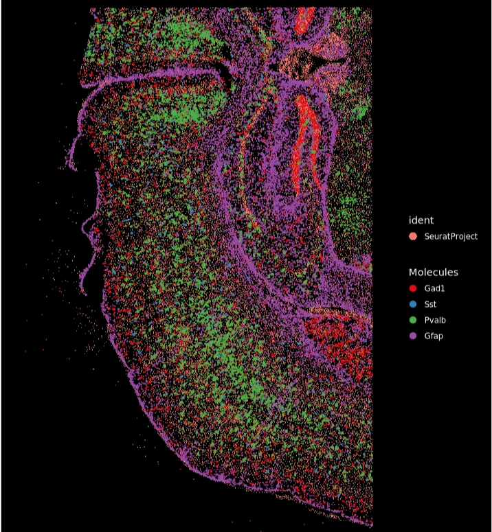
空间图显示所选基因的单个RNA分子的位置

可视化基因表达与裁剪ROI

空间绘制基因表达水平，类似于 FeaturePlot。调整 max.cutoff 以获得更好的对比度。

ImageFeaturePlot(xenium.obj, features = c("Cux2", "Rorb", "Bcl11b", "Foxp2"),
                 max.cutoff = c(25, 35, 12, 10), size = 0.75, cols = c("white", "red"))
# 或者使用 'q90' 代表90分位数: max.cutoff = "q90"

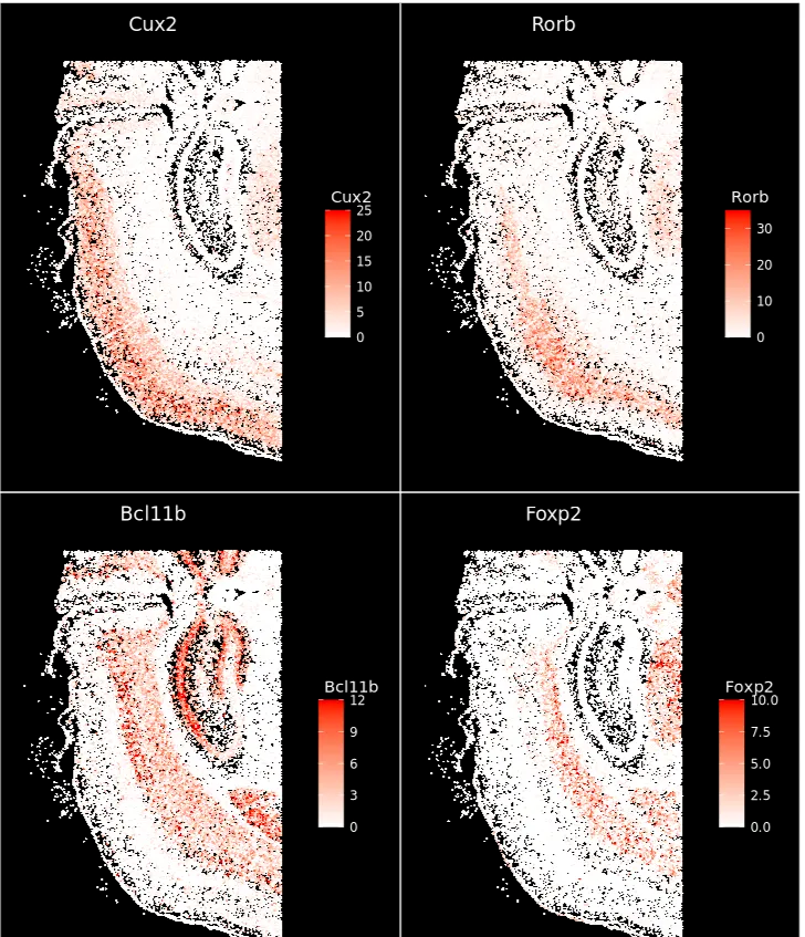
空间图，细胞根据指定分层标记基因的表达量着色

使用 Crop()放大到感兴趣区域(ROI)。

cropped.coords <- Crop(xenium.obj[["fov"]], x = c(1200, 2900), y = c(3750, 4550), coords = "plot")
xenium.obj[["zoom"]] <- cropped.coords

可视化裁剪区域

现在可视化裁剪区域的细胞分割边界和选定的分子。

DefaultBoundary(xenium.obj[["zoom"]]) <- "segmentation"
ImageDimPlot(xenium.obj, fov = "zoom", axes = TRUE, border.color = "white",
             border.size = 0.1, cols = "polychrome", coord.fixed = FALSE,
             molecules = c("Gad1", "Sst", "Npy2r", "Pvalb", "Nrn1"), nmols = 10000)

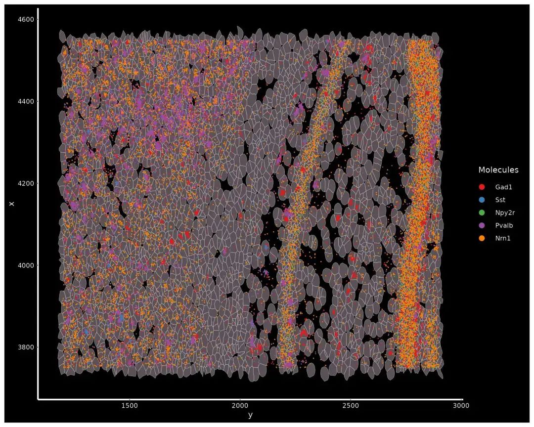
放大的空间图，显示细胞边界和所选基因的分子位置

标准化、降维与聚类

标准Seurat流程：SCTransform, PCA, UMAP, FindNeighbors, FindClusters。(此步骤约需5分钟)

xenium.obj <- SCTransform(xenium.obj, assay = "Xenium", verbose = FALSE)
xenium.obj <- RunPCA(xenium.obj, npcs = 30, features = rownames(xenium.obj), verbose = FALSE)
xenium.obj <- RunUMAP(xenium.obj, dims = 1:30, verbose = FALSE)
xenium.obj <- FindNeighbors(xenium.obj, reduction = "pca", dims = 1:30, verbose = FALSE)
xenium.obj <- FindClusters(xenium.obj, resolution = 0.3, verbose = FALSE)

在UMAP空间和空间图像上可视化聚类。

DimPlot(xenium.obj)

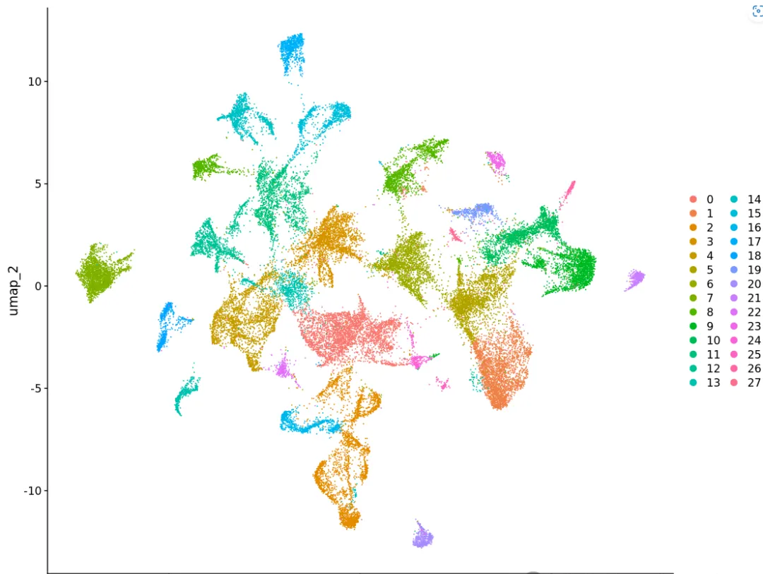
UMAP图，细胞根据聚类身份着色

ImageDimPlot(xenium.obj, cols = "polychrome", size = 0.75) 
#ImageDimPlot：显示区域的分子和细胞分布

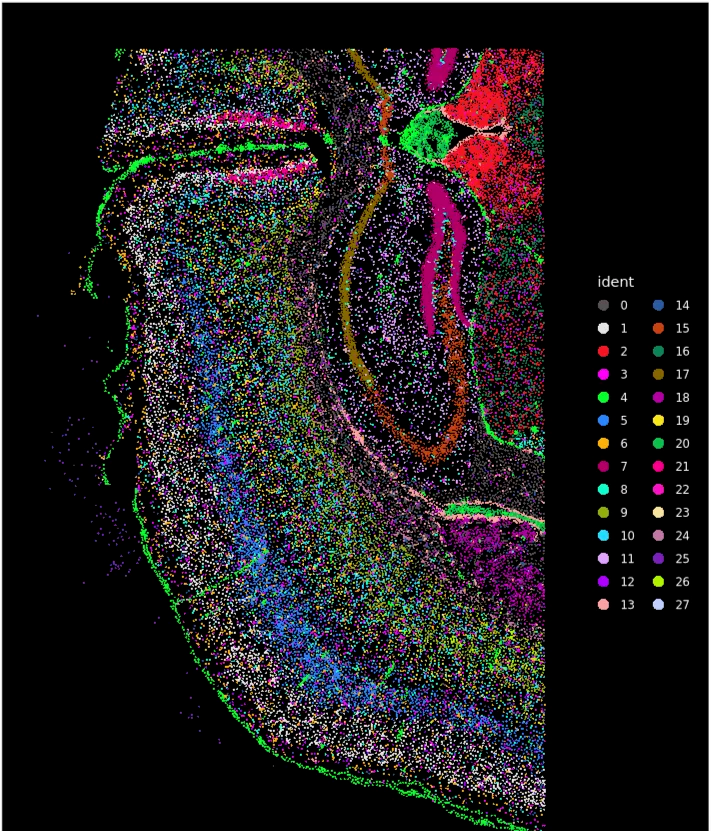
空间图，细胞根据聚类身份着色

在UMAP上检查标记基因的表达。

p1 <- ImageFeaturePlot(xenium.obj, features = "Bcl11b", axes = TRUE, max.cutoff = "q90")
p1
#ImageFeaturePlot：展示特定基因（如Bcl11b）在空间上的表达分布（颜色表示表达量）

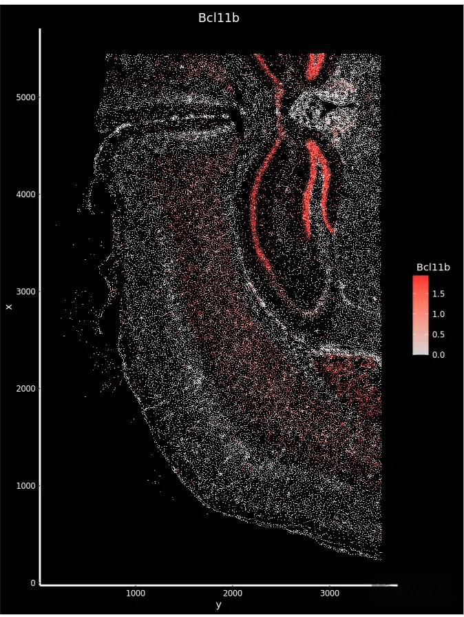
UMAP图，显示标记基因的表达水平

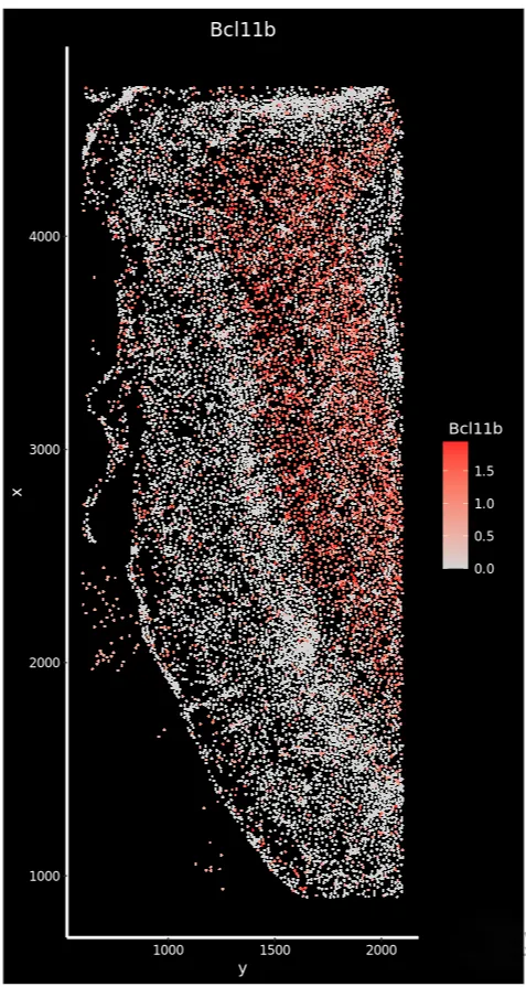
提取裁剪区域数据

crop <- Crop(xenium.obj[["fov"]], x = c(600, 2100), y = c(900, 4700)) 
xenium.obj[["crop"]] <- crop #进一步裁剪数据以提取感兴趣的区域 
p2 <- ImageFeaturePlot(xenium.obj, fov = "crop", features = "Bcl11b", size = 1, axes = TRUE, max.cutoff = "q90") 
p2

裁剪皮层区域并准备细胞类型注释 (RCTD)

为了使用Allen脑图谱参考进行注释，首先使用 Slc17a7 (兴奋性神经元标记) 的表达作为指导，裁剪出皮层区域。

# 重新加载原始对象以进行精确裁剪（如果需要）
# xenium.obj <- LoadXenium(path, fov = "fov")
# 可视化 Slc17a7 以指导裁剪坐标
# ImageFeaturePlot(xenium.obj, fov="fov", features = "Slc17a7", axes = TRUE, max.cutoff = "q90")

# 已确定坐标：
crop <- Crop(xenium.obj[["fov"]], x = c(600, 2100), y = c(900, 4700))
xenium.obj[["cortex_crop"]] <- crop # 使用新名称以避免与之前的 "crop" 冲突

# 安装用于RCTD的spacexr包
# devtools::install_github("dmcable/spacexr", build_vignettes = FALSE)
library(spacexr)

# 为RCTD准备数据
query.counts <- GetAssayData(xenium.obj, assay = "Xenium", slot = "counts")[, Cells(xenium.obj[["cortex_crop"]])]
coords <- GetTissueCoordinates(xenium.obj[["cortex_crop"]], which = "centroids")
rownames(coords) <- coords$cell
coords$cell <- NULL # Seurat v5 GetTissueCoordinates 返回一个包含 cell 列的 data.frame
query <- SpatialRNA(coords, query.counts, colSums(query.counts))

下载并加载Allen皮层参考数据 (参考教程获取URL: dropbox.com/s/cuowvm4vrf65pvq/allen_cortex.rds?dl=1)
allen.cortex.ref <- readRDS("/你的路径/allen_cortex.rds")
allen.cortex.ref <- UpdateSeuratObject(allen.cortex.ref)
Idents(allen.cortex.ref) <- "subclass"
allen.cortex.ref <- subset(allen.cortex.ref, subset = subclass != "CR") # 移除稀有细胞类型
counts_ref <- GetAssayData(allen.cortex.ref, assay = "RNA", slot = "counts")
cluster_ref <- as.factor(allen.cortex.ref$subclass)
names(cluster_ref) <- colnames(allen.cortex.ref)
nUMI_ref <- colSums(counts_ref) # 或 allen.cortex.ref$nCount_RNA
levels(cluster_ref) <- gsub("/", "-", levels(cluster_ref))
reference <- Reference(counts_ref, cluster_ref, nUMI_ref)

运行RCTD并添加注释

# 'reference' 对象已按教程准备好
RCTD <- create.RCTD(query, reference, max_cores = 8) # 使用适当的核心数
RCTD <- run.RCTD(RCTD, doublet_mode = "doublet")
annotations.df <- RCTD@results$results_df
annotations <- annotations.df$first_type
names(annotations) <- rownames(annotations.df)

#将注释添加到Seurat对象中 (如果未运行RCTD，则为示例模拟注释)
xenium.obj$predicted.celltype.cortex <- NA # 初始化列
common_cells <- intersect(Cells(xenium.obj[["cortex_crop"]]), names(annotations))
xenium.obj$predicted.celltype.cortex[common_cells] <- annotations[common_cells]
xenium.obj.cortex_annotated <- subset(xenium.obj, cells = common_cells[!is.na(xenium.obj$predicted.celltype.cortex[common_cells])])

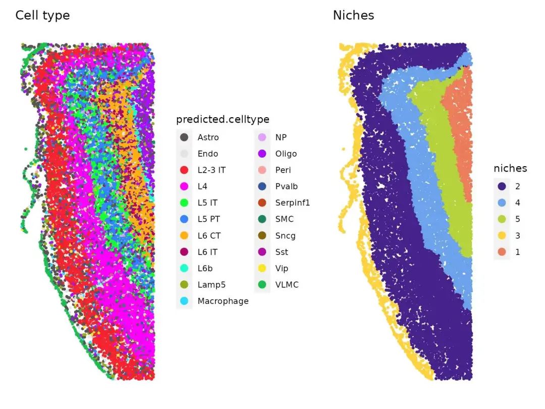
空间生态位 (Niche) 分析

通过空间上相邻细胞类型的组成来定义组织区域 ("niches")。使用 cortex_crop FOV和来自RCTD的 predicted.celltype.cortex。

# 确保预测的细胞类型存在于 `cortex_crop` FOV的细胞上
# ( xenium.obj.cortex_annotated 或 xenium.obj 已经有了 predicted.celltype.cortex 列，
# 并且我们只对 cortex_crop FOV 中的细胞进行操作)
#  xenium.obj 已经有了 predicted.celltype.cortex 列，并且我们只对 cortex_crop FOV 中的细胞进行操作
# xenium.obj <- BuildNicheAssay(object = xenium.obj, fov = "cortex_crop",
#                               group.by = "predicted.celltype.cortex", # 此列存在于RCTD步骤之后
#                               niches.k = 5, neighbors.k = 30)

可视化细胞类型与生态位。

# 确保 'predicted.celltype.cortex' 和 'niches' 在对象的元数据中，针对 fov='cortex_crop'
celltype.plot <- ImageDimPlot(xenium.obj, fov = "cortex_crop", group.by = "predicted.celltype.cortex",
                              size = 1.5, cols = "polychrome", dark.background = FALSE) + ggtitle("细胞类型")
niche.plot <- ImageDimPlot(xenium.obj, fov = "cortex_crop", group.by = "niches", size = 1.5,
                            dark.background = FALSE) + ggtitle("生态位 (Niches)") +
                           scale_fill_manual(values = c("#442288", "#6CA2EA", "#B5D33D", "#FED23F", "#EB7D5B")) # 示例颜色
print(celltype.plot | niche.plot)