空间转录组: 反卷积及可视化

数据科学工厂

发布于 2025-09-17 14:51:24

5700

代码可运行

文章被收录于专栏：数据科学（冷冻工厂）数据科学（冷冻工厂）

运行总次数：0

代码可运行

引言

本系列讲解 空间转录组学 (Spatial Transcriptomics) 相关基础知识与数据分析教程[1]，持续更新，欢迎关注，转发，文末有交流群！

RCTD

接下来，我们使用 spacexr（也称为 RCTD）进行反卷积。默认情况下，runRctd() 的 rctd_mode = "doublet" 指定最多两个亚群共存于一个数据单元（即一个 spot）中；在此，我们将 rctd_mode 设置为 "full"，以允许拟合任意数量的亚群。

rctd_data <- createRctd(vis, sce, cell_type_col = "Annogrp")
(res <- runRctd(rctd_data, max_cores = 4, rctd_mode = "full"))

##  class: SpatialExperiment 
##  dim: 12 4962 
##  metadata(4): spatial_rna config cell_type_info internal_vars
##  assays(1): weights
##  rownames(12): B DCIS1 ... stromal tumor
##  rowData names(0):
##  colnames(4962): AACACCTACTATCGAA-1 AACACGTGCATCGCAC-1 ...
##    TGTTGGCCAGACCTAC-1 TGTTGGCCTACACGTG-1
##  colData names(1): sample_id
##  reducedDimNames(0):
##  mainExpName: NULL
##  altExpNames(0):
##  spatialCoords names(2) : x y
##  imgData names(0):

由 RCTD 推断的权重应进行归一化，使得每个 spot 的细胞类型比例之和为 1：

# scale weights such that they sum to 1
ws <- assay(res)
ws <- sweep(ws, 2, colSums(ws), `/`)

ws_rctd <- data.frame(t(as.matrix(ws)))
ws_rctd[1:5, 1:5] |> round(2)

##                        B DCIS1 DCIS2    T dendritic
##  AACACCTACTATCGAA-1 0.00  0.00  0.00 0.00      0.01
##  AACACGTGCATCGCAC-1 0.04  0.01  0.00 0.04      0.00
##  AACACTTGGCAAGGAA-1 0.00  0.00  0.03 0.01      0.01
##  AACAGGAAGAGCATAG-1 0.03  0.00  0.00 0.08      0.03
##  AACAGGATTCATAGTT-1 0.00  0.00  0.01 0.00      0.00

# add proportion estimates to colData
colData(vis)[names(ws_rctd)] <- ws_rctd[colnames(vis), ]

CARD

另一种可用的方法是 CARD。首先，我们重命名 CARD 的空间坐标列。

# realize the delayed matrices, as CARD do not support delayed matrix handling yet
counts(sce) <- as(counts(sce), "sparseMatrix")
counts(vis) <- as(counts(vis), "sparseMatrix")
colnames(spatialCoords(vis)) <- c("x", "y")

接下来，我们执行 CARD 反卷积。在此，我们展示了 CARD 与 SingleCellExperiment 和 SpatialExperiment 的互操作性。反卷积结果矩阵已归一化，使得每个 spot 的细胞类型比例之和等于 1。

set.seed(2025)
CARD_obj <- CARD_deconvolution(
    spe = vis,
    sce = sce,
    sc_count = NULL,
    sc_meta = NULL,
    spatial_count = NULL,
    spatial_location = NULL,
    ct_varname = "Annogrp",
    ct_select = NULL,       # decon with all sce$Annogrp cell types
    sample_varname = NULL,  # use all sce as one ref sample 
    mincountgene = 100,
    mincountspot = 5
)
ws_card <- CARD_obj$Proportion_CARD
# order cell type names alphabetically, as for RCTD
ws_card <- data.frame(ws_card[, colnames(ws_rctd)])

ws_card[1:5, 1:5] |> round(2)

##                     B DCIS1 DCIS2    T dendritic
##  AACACCTACTATCGAA-1 0     0     0 0.00         0
##  AACACGTGCATCGCAC-1 0     0     0 0.00         0
##  AACACTTGGCAAGGAA-1 0     0     0 0.01         0
##  AACAGGAAGAGCATAG-1 0     0     0 0.02         0
##  AACAGGATTCATAGTT-1 0     0     0 0.00         0

可视化

首先，我们定义了几个附件功能。

.plt_xy <- \(ws, vis, col, point_size) {
    xy <- spatialCoords(vis)[rownames(ws), ]
    colnames(xy) <- c("x", "y")
    df <- cbind(ws, xy)
    ggplot(df, aes(x, y, col=.data[[col]])) + 
        coord_equal() + theme_void() + 
        geom_point(size = point_size)
}

.plt_decon <- \(ws, vis){
    lapply(names(ws), \(.) 
      .plt_xy(ws, vis, col = ., point_size = 0.3)) |> 
      wrap_plots(nrow = 3) & theme(
      legend.key.width = unit(0.5, "lines"),
      legend.key.height = unit(1, "lines")) &
      scale_color_gradientn(colors = pals::jet())
}

我们可以在 x-y 空间中对反卷积权重进行可视化，即按照估计落入某个 spot 的给定细胞类型的比例进行着色：

.plt_decon(ws = ws_rctd, vis)

.plt_decon(ws = ws_card, vis)

反卷积结果也可以以热图形式查看，其中行 = 细胞，列 = 聚类：

plot_heat_ws <- function(ws, string){
    p <- pheatmap(ws, show_rownames = FALSE, show_colnames = TRUE, main=string,
                  cellwidth = 12, treeheight_row = 5, treeheight_col = 5)
    return(p)
}
plot_heat_ws(ws_rctd, string="RCTD") 
plot_heat_ws(ws_card, string="CARD")

在两种方法中，我们都观察到超过一半的 spot 被估计具有超过 50 % 的 stromal 比例。少数 spot 对癌性子群体 DCIS1 和 DCIS2 表现出强烈且独特的信号。

为了与 10x Genomics 提供的 spot 注释进行比较，我们纳入了由 RCTD 反卷积得出的细胞类型。

ws <- ws_rctd
# derive majority vote label
ids <- names(ws)[apply(ws, 1, which.max)]
names(ids) <- rownames(ws)
vis$RCTD <- factor(ids[colnames(vis)])

# derive majority vote excluding stromal cells
ws_no_stroma <- ws[, colnames(ws) != "stromal"]
ids_no_stroma <- names(ws_no_stroma)[apply(ws_no_stroma, 1, which.max)]
names(ids_no_stroma) <- rownames(ws)
vis$RCTD_no_stroma <- factor(ids_no_stroma[colnames(vis)])

我们可以在空间上可视化这三个注释：

lapply(c("anno", "RCTD", "RCTD_no_stroma"), 
       \(.) plotCoords(vis, annotate=.)) |>
    wrap_plots(nrow = 1) &
    theme(legend.key.size = unit(0, "lines")) &
    scale_color_manual(values = unname(pals::trubetskoy()))

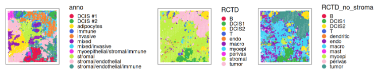
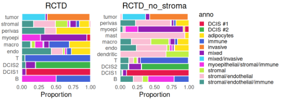
请注意强烈的 stromal 信号，以及 macrophages 是 stromal 细胞中第二常见的细胞类型。为了帮助表征来自反卷积的亚群，我们可以将它们的空间分布与提供的注释进行对比查看：

cd <- data.frame(colData(vis))
df <- as.data.frame(with(cd, table(RCTD, anno)))
fd <- as.data.frame(with(cd, table(RCTD_no_stroma, anno)))
ggplot(df, aes(Freq, RCTD, fill = anno)) + ggtitle("RCTD") +
    ggplot(fd, aes(Freq, RCTD_no_stroma, fill = anno)) + ggtitle("RCTD_no_stroma") +
    plot_layout(nrow = 1, guides = "collect") &
    labs(x = "Proportion", y = NULL) &
    coord_cartesian(expand = FALSE) &
    geom_col(width = 1, col = "white", position = "fill") &
    scale_fill_manual(values = unname(pals::trubetskoy())) &
    theme_minimal() & theme(aspect.ratio = 1,
                            legend.key.size = unit(2/3, "lines"),
                            plot.title = element_text(hjust=0.5))

接下来，我们可以探究所提供的注释与两种反卷积标签之间的一致性。

hm <- \(mat, string) pheatmap(
    mat, show_rownames = TRUE, show_colnames = TRUE, main=string,
    cellwidth = 10, cellheight = 10, treeheight_row = 5, treeheight_col = 5)
hm(prop.table(table(vis$anno, vis$RCTD), 2), string="RCTD")
hm(prop.table(table(vis$anno, vis$RCTD_no_stroma), 2), string="RCTD_no_stroma")

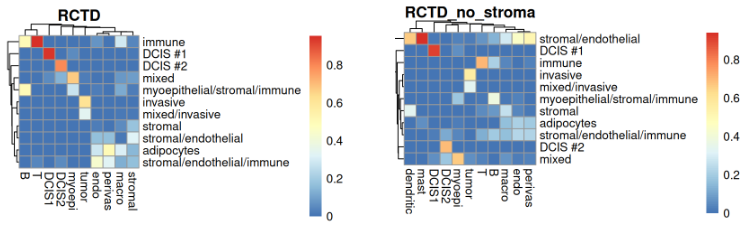
总体而言，我们观察到所提供的 spot 标签与 RCTD 反卷积得出的注释之间存在一致性。

在清除 stromal 之前，某些免疫细胞类型（如 dendritic 和 mast）从未有机会获得最高的细胞类型比例。在左图中，在 RCTD 注释为 T 细胞的所有 spot 中，几乎所有这些 spot 在提供的注释中都属于 “immune” 类型。对于标注为 “DCIS1”、“DCIS2” 和 “Invasive tumor” 的 spot，也观察到高度一致。

总之，基于反卷积的细胞类型比例估计能够重现 PCs，进而重现表达变异性。

未完待续，欢迎关注！

Reference

[1]

Ref: https://lmweber.org/OSTA/

本文参与腾讯云自媒体同步曝光计划，分享自微信公众号。

原始发表：2025-09-09，如有侵权请联系 cloudcommunity@tencent.com 删除

教程