R语言中基于混合数据抽样(MIDAS)回归的HAR-RV模型预测GDP增长

拓端

发布于 2025-05-15 13:01:47

11400

代码可运行

文章被收录于专栏：拓端tecdat拓端tecdat

运行总次数：0

代码可运行

原文链接：http://tecdat.cn/?p=12292

我们复制了Ghysels（2013）中提供的示例。我们进行了MIDAS回归分析，来预测季度GDP增长以及每月非农就业人数的增长（点击文末“阅读原文”获取完整代码数据）。

相关视频

预测GDP增长

预测公式如下

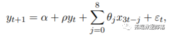
其中yt是按季度季节性调整后的实际GDP的对数增长，x3t是月度总就业非农业工资的对数增长。

首先，我们加载数据并执行转换。

R> y <- window(USqgdp, end = c(2011, 2))
R> x <- window(USpayems, end = c(2011, 7))
R> yg <- diff(log(y)) * 100
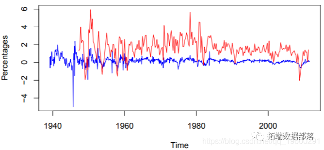
R> xg <- diff(log(x)) * 100

最后两行用于均衡样本大小，样本大小在原始数据中有所不同。我们只需在数据的开头和结尾添加其他NA值即可。数据的图形表示如图所示。要指定midas_r函数的模型，我们以下等效形式重写它：

点击标题查阅往期内容

就像在Ghysels（2013）中一样，我们将估算样本限制在1985年第一季度到2009年第一季度之间。我们使用Beta多项式，非零Beta和U-MIDAS权重来评估模型。

R> coef(beta0)
(Intercept) yy xx1 xx2 xx3
0.83152740.10589102.58871031.020120213.6867809

R> coef(betan)
(Intercept) yy xx1 xx2 xx3 xx4
0.937787050.067481412.269706460.986591741.49616336 -0.09184983

(Intercept) yy xx1 xx2 xx3 xx4
0.929897570.083583932.000472050.881345970.42964662 -0.17596814
xx5 xx6 xx7 xx8 xx9
0.283510101.16285271 -0.53081967 -0.73391876 -1.18732001

我们可以使用2009年第2季度至2011年第2季度包含9个季度的样本数据评估这三个模型的预测性能。

R> fulldata <- list(xx = window(nx, start = c(1985, 1), end = c(2011, 6)),
+ yy = window(ny, start = c(1985, 1), end = c(2011, 2)))
R> insample <- 1:length(yy)
R> outsample <- (1:length(fulldata$yy))\[-insample\]
R> avgf <- average_forecast(list(beta0, betan, um), data = fulldata,
+ insample = insample, outsample = outsample)
R> sqrt(avgf$accuracy$individual$MSE.out.of.sample)
\[1\] 0.5361953 0.4766972 0.4457144

我们看到，MIDAS回归模型提供了最佳的样本外RMSE。

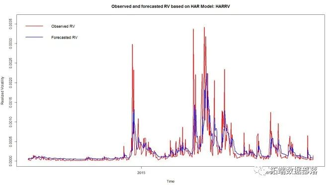
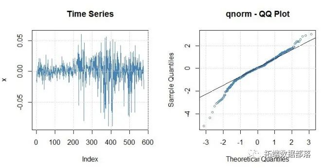
预测实际波动

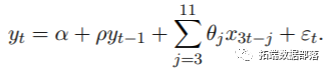
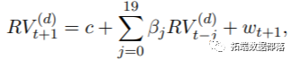
作为另一个演示，我们使用midasr来预测每日实现的波动率。Corsi（2009）提出了一个简单的预测每日实际波动率的模型。实现波动率的异质自回归模型（HAR-RV）定义为

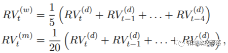
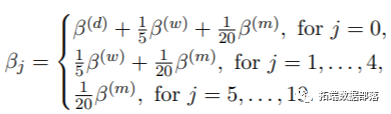
我们假设一周有5天，一个月有4周。该模型是MIDAS回归的特例：

为了进行经验论证，我们使用了由Heber，Lunde，Shephard和Sheppard（2009）提供的关于股票指数的已实现波动数据。我们基于5分钟的收益数据估算S＆P500指数的年度实现波动率模型。

 Parameters:
Estimate Std. Error t value Pr(>|t|)
(Intercept) 0.83041 0.36437 2.279 0.022726 *
rv1 0.34066 0.04463 7.633 2.95e-14 ***
rv2 0.41135 0.06932 5.934 3.25e-09 ***
rv3 0.19317 0.05081 3.802 0.000146 ***
\-\-\-
Signif. codes: 0 '***' 0.001 '**' 0.01 '*' 0.05 '.' 0.1 ' ' 1
Residual standard error: 5.563 on 3435 degrees of freedom

为了进行比较，我们还使用归一化指数Almon权重来估计模型

 Parameters:
Estimate Std. Error t value Pr(>|t|)
(Intercept) 0.837660 0.377536 2.219 0.0266 *
rv1 0.944719 0.027748 34.046 < 2e-16 ***
rv2 -0.768296 0.096120 -7.993 1.78e-15 ***
rv3 0.029084 0.005604 5.190 2.23e-07 ***
\-\-\-
Signif. codes: 0 '***' 0.001 '**' 0.01 '*' 0.05 '.' 0.1 ' ' 1
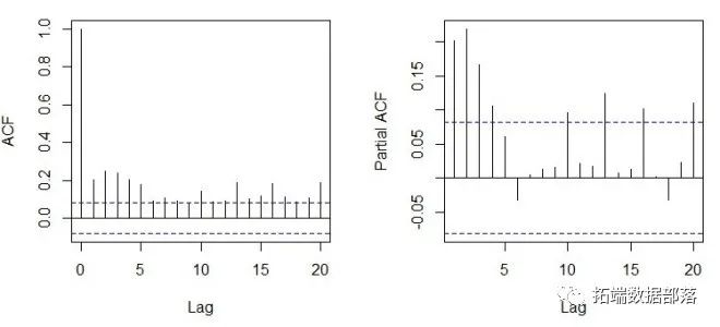
Residual standard error: 5.535 on 3435 degrees of freedom

我们可以使用异方差性和自相关鲁棒权重规范检验hAhr_test来检验这些限制中哪些与数据兼容。

 hAh restriction test (robust version)
data:
hAhr = 28.074, df = 17, p-value = 0.04408
 
hAh restriction test (robust version)
data:
hAhr = 19.271, df = 17, p-value = 0.3132

我们可以看到，与MIDAS回归模型中的HAR-RV隐含约束有关的零假设在0.05的显着性水平上被拒绝，而指数Almon滞后约束的零假设则不能被拒绝。

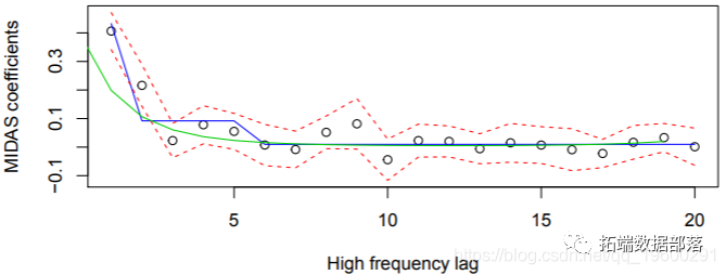
图说明了拟合的MIDAS回归系数和U-MIDAS回归系数及其相应的95％置信区间。对于指数Almon滞后指标，我们可以通过AIC或BIC选择滞后次数。

我们使用了两种优化方法来提高收敛性。将测试函数应用于每个候选模型。函数hAhr_test需要大量的计算时间，尤其是对于滞后阶数较大的模型，因此我们仅在第二步进行计算，并且限制了滞后 restriction test 的选择。AIC选择模型有9阶滞后：

 Selected model with AIC = 21551.97
Based on restricted MIDAS regression model
The p-value for the null hypothesis of the test hAhr_test is0.5531733
 Parameters:
Estimate Std. Error t value Pr(>|t|)
(Intercept) 0.961020.369442.6010.00933 **
rv1 0.937070.0272934.337 < 2e-16 ***
rv2 -1.192330.19288 -6.1827.08e-10 ***
rv3 0.096570.021904.4111.06e-05 ***
\-\-\-
Signif. codes: 0'***'0.001'**'0.01'*'0.05'.'0.1' '1
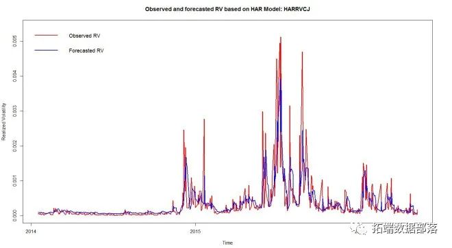
Residual standard error: 5.524on3440 degrees of freedom

hAh_test的HAC再次无法拒绝指数Almon滞后的原假设。我们可以使用具有1000个观测值窗口的滚动预测来研究两个模型的预测性能。为了进行比较，我们还计算了无限制AR（20）模型的预测。

 Model MSE.out.of.sample MAPE.out.of.sample
1 rv ~  (rv, 1:20, 1) 10.8251626.60201
2 rv ~  (rv, 1:20, 1, harstep) 10.4584225.93013
3 rv ~  (rv, 1:9, 1, nealmon) 10.3479725.90268
MASE.out.of.sample MSE.in.sample MAPE.in.sample MASE.in.sample
10.819956628.6160221.567040.8333858
20.801968729.2498921.592200.8367377
30.794512129.0828421.814840.8401646

我们看到指数Almon滞后模型略优于HAR-RV模型，并且两个模型均优于AR（20）模型。