CUT&Tag 数据处理和分析教程（5）

数据科学工厂

发布于 2025-04-04 08:16:41

14900

代码可运行

文章被收录于专栏：数据科学（冷冻工厂）数据科学（冷冻工厂）

运行总次数：0

代码可运行

引言

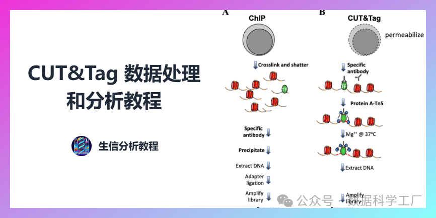
本系列[1] 将开展全新的CUT&Tag 数据处理和分析专栏。

重复去除

CUT&Tag 技术会将接头序列插入到抗体连接的 pA-Tn5 附近的 DNA 中，而插入的具体位置会受到周围 DNA 可及性的影响。因此，那些起始和结束位置完全相同的片段是比较常见的，但这些所谓的“重复项”可能并不是由于 PCR 过程中的复制产生的。实际上，发现高质量的 CUT&Tag 数据集的表观重复率通常很低，即使是看起来像是“重复”的片段，也可能是真实的片段。因此，不建议删除这些重复项。不过，在实验样本量极少，或者怀疑存在 PCR 扩增重复的情况下，可以考虑删除重复项。以下命令展示了如何使用 Picard 来检查重复率。

##== linux command ==##
## depending on how you load picard and your server environment, the picardCMD can be different. Adjust accordingly.
picardCMD="java -jar picard.jar"
mkdir -p $projPath/alignment/removeDuplicate/picard_summary

## Sort by coordinate
$picardCMD SortSam I=$projPath/alignment/sam/${histName}_bowtie2.sam O=$projPath/alignment/sam/${histName}_bowtie2.sorted.sam SORT_ORDER=coordinate

## mark duplicates
$picardCMD MarkDuplicates I=$projPath/alignment/sam/${histName}_bowtie2.sorted.sam O=$projPath/alignment/removeDuplicate/${histName}_bowtie2.sorted.dupMarked.sam METRICS_FILE=$projPath/alignment/removeDuplicate/picard_summary/${histName}_picard.dupMark.txt

## remove duplicates
picardCMD MarkDuplicates I=$projPath/alignment/sam/${histName}_bowtie2.sorted.sam O=$projPath/alignment/removeDuplicate/${histName}_bowtie2.sorted.rmDup.sam REMOVE_DUPLICATES=true METRICS_FILE=$projPath/alignment/removeDuplicate/picard_summary/${histName}_picard.rmDup.txt

总结了明显的重复率，并计算出唯一的库大小而无需重复。

##=== R command ===## 
## Summarize the duplication information from the picard summary outputs.
dupResult = c()
for(hist in sampleList){
  dupRes = read.table(paste0(projPath, "/alignment/removeDuplicate/picard_summary/", hist, "_picard.rmDup.txt"), header = TRUE, fill = TRUE)
  
  histInfo = strsplit(hist, "_")[[1]]
  dupResult = data.frame(Histone = histInfo[1], Replicate = histInfo[2], MappedFragNum_hg38 = dupRes$READ_PAIRS_EXAMINED[1] %>% as.character %>% as.numeric, DuplicationRate = dupRes$PERCENT_DUPLICATION[1] %>% as.character %>% as.numeric * 100, EstimatedLibrarySize = dupRes$ESTIMATED_LIBRARY_SIZE[1] %>% as.character %>% as.numeric) %>% mutate(UniqueFragNum = MappedFragNum_hg38 * (1-DuplicationRate/100))  %>% rbind(dupResult, .)
}
dupResult$Histone = factor(dupResult$Histone, levels = histList)
alignDupSummary = left_join(alignSummary, dupResult, by = c("Histone", "Replicate", "MappedFragNum_hg38")) %>% mutate(DuplicationRate = paste0(DuplicationRate, "%"))
alignDupSummary

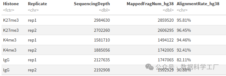
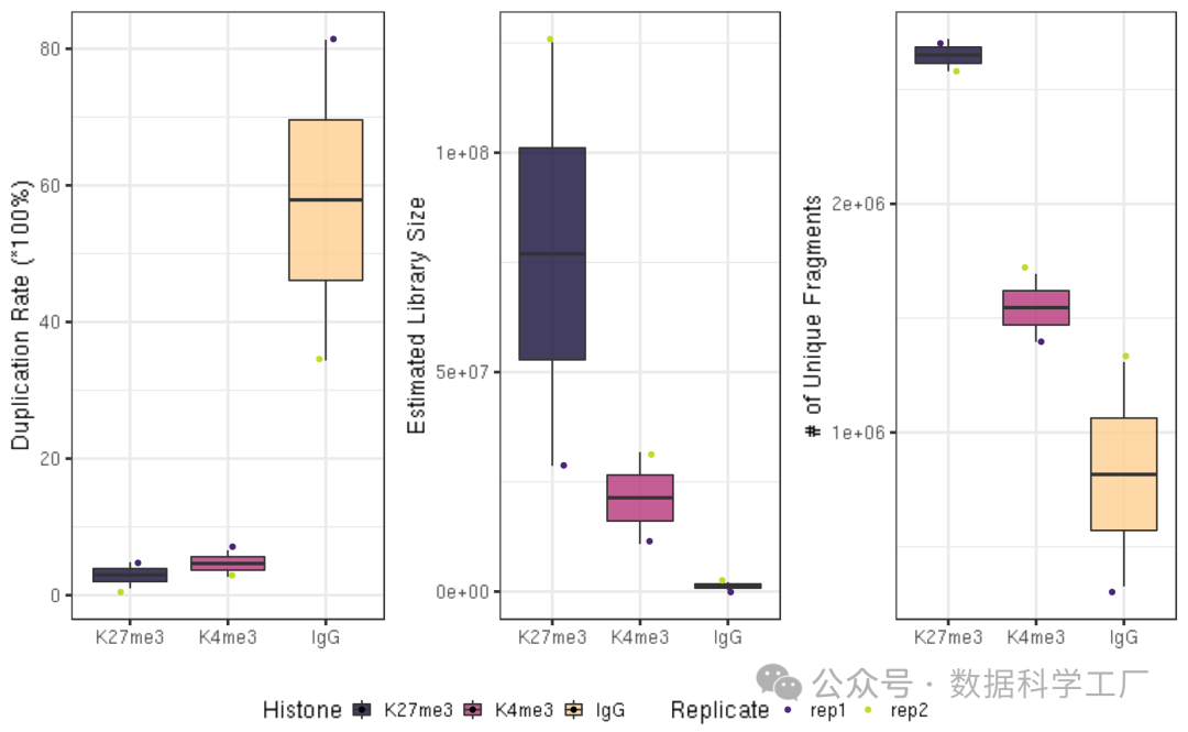
在这些示例数据集中，IgG 对照样本的重复率比较高。这是因为这些样本中的数据来源于 CUT&Tag 反应中的非特异性片段化。因此，在进行下游分析之前，从 IgG 数据集中去除重复项是比较合理的。
估计的文库大小是根据 Picard 计算的 PE 重复率来估算文库中独特分子数量的。
估计的文库大小与目标表位的丰度以及抗体的质量成正比，而 IgG 样本的估计文库大小通常会很低。
独特片段数是通过公式 MappedFragNum_hg38 * (1 - DuplicationRate/100) 计算得出的。

##=== R command ===## 
## generate boxplot figure for the  duplication rate
fig4A = dupResult %>% ggplot(aes(x = Histone, y = DuplicationRate, fill = Histone)) +
    geom_boxplot() +
    geom_jitter(aes(color = Replicate), position = position_jitter(0.15)) +
    scale_fill_viridis(discrete = TRUE, begin = 0.1, end = 0.9, option = "magma", alpha = 0.8) +
    scale_color_viridis(discrete = TRUE, begin = 0.1, end = 0.9) +
    theme_bw(base_size = 18) +
    ylab("Duplication Rate (*100%)") +
    xlab("") 

fig4B = dupResult %>% ggplot(aes(x = Histone, y = EstimatedLibrarySize, fill = Histone)) +
    geom_boxplot() +
    geom_jitter(aes(color = Replicate), position = position_jitter(0.15)) +
    scale_fill_viridis(discrete = TRUE, begin = 0.1, end = 0.9, option = "magma", alpha = 0.8) +
    scale_color_viridis(discrete = TRUE, begin = 0.1, end = 0.9) +
    theme_bw(base_size = 18) +
    ylab("Estimated Library Size") +
    xlab("") 

fig4C = dupResult %>% ggplot(aes(x = Histone, y = UniqueFragNum, fill = Histone)) +
    geom_boxplot() +
    geom_jitter(aes(color = Replicate), position = position_jitter(0.15)) +
    scale_fill_viridis(discrete = TRUE, begin = 0.1, end = 0.9, option = "magma", alpha = 0.8) +
    scale_color_viridis(discrete = TRUE, begin = 0.1, end = 0.9) +
    theme_bw(base_size = 18) +
    ylab("# of Unique Fragments") +
    xlab("")

ggarrange(fig4A, fig4B, fig4C, ncol = 3, common.legend = TRUE, legend="bottom")