【机器学习与实现】kNN分类算法示例


一、混淆矩阵相关概念示例
from sklearn.metrics import confusion_matrix,accuracy_score,precision_score,recall_score,f1_score
from sklearn.metrics import classification_report
y_true = [1, 1, 0, 1, 0, 1, 0, 1, 1, 0, 0, 0]
y_pred = [1, 0, 1, 0, 1, 1, 1, 1, 0, 0, 1, 0]
#使用help(confusion_matrix)命令,可以查看混淆矩阵的联机帮助
#在该联机帮助的示例中,是把1看作Positive,把0看作Negative,并且混淆矩阵的右下角是tp
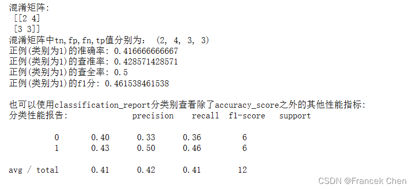
print("混淆矩阵:\n",confusion_matrix(y_true,y_pred))
tn,fp,fn,tp=confusion_matrix(y_true,y_pred).ravel()
print("混淆矩阵中tn,fp,fn,tp值分别为:",(tn,fp,fn,tp))
print("正例(类别为1)的准确率:",accuracy_score(y_true,y_pred))
print("正例(类别为1)的查准率:",precision_score(y_true, y_pred))
print("正例(类别为1)的查全率:",recall_score(y_true, y_pred))
print("正例(类别为1)的f1分:",f1_score(y_true, y_pred))
print("\n也可以使用classification_report分类别查看除了accuracy_score之外的其他性能指标:")
print("分类性能报告:",classification_report(y_true, y_pred, labels=[0,1]))对比上述输出结果,可以发现:
accuracy_score/precision_score/recall_score/f1_score函数只显示正例 (类别为1) 的性能指标;
而classification_report既可以显示正例(类别为1)、还可以显示出反例 (类别为0) 的性能指标。
对上面运行结果的分析如下图所示:
y_true = [1, 1, 0, 1, 0, 1, 0, 1, 1, 0, 0, 0]
y_pred = [1, 0, 1, 0, 1, 1, 1, 1, 0, 0, 1, 0]
查准率和查全率是一对矛盾的度量,一般来说,查准率高时,查全率往往会偏低,查全率高时,查准率往往会偏低。而F1-Score指标综合了Precision与Recall的产出的结果,是F1是基于查准率与查重率的调和平均。F1-Score的取值范围从0到1,1代表模型的输出最好,0代表模型的输出结果最差。
二、使用kNN(k近邻)算法对鸢尾花数据集进行分类
(一)加载并查看鸢尾花数据集
参考资源: https://blog.csdn.net/weixin_45014385/article/details/123618841 https://www.cnblogs.com/gemine/p/11130032.html
from sklearn.datasets import load_iris
#加载sklearn自带的鸢尾花数据集
iris = load_iris()
#查看该数据集的说明信息,该说明信息是一个字典
iris{'DESCR': 'Iris Plants Database\n====================\n\nNotes\n-----\nData Set Characteristics:\n :Number of Instances: 150 (50 in each of three classes)\n :Number of Attributes: 4 numeric, predictive attributes and the class\n :Attribute Information:\n - sepal length in cm\n - sepal width in cm\n - petal length in cm\n - petal width in cm\n - class:\n - Iris-Setosa\n - Iris-Versicolour\n - Iris-Virginica\n :Summary Statistics:\n\n ============== ==== ==== ======= ===== ====================\n Min Max Mean SD Class Correlation\n ============== ==== ==== ======= ===== ====================\n sepal length: 4.3 7.9 5.84 0.83 0.7826\n sepal width: 2.0 4.4 3.05 0.43 -0.4194\n petal length: 1.0 6.9 3.76 1.76 0.9490 (high!)\n petal width: 0.1 2.5 1.20 0.76 0.9565 (high!)\n ============== ==== ==== ======= ===== ====================\n\n :Missing Attribute Values: None\n :Class Distribution: 33.3% for each of 3 classes.\n :Creator: R.A. Fisher\n :Donor: Michael Marshall (MARSHALL%PLU@io.arc.nasa.gov)\n :Date: July, 1988\n\nThis is a copy of UCI ML iris datasets.\nhttp://archive.ics.uci.edu/ml/datasets/Iris\n\nThe famous Iris database, first used by Sir R.A Fisher\n\nThis is perhaps the best known database to be found in the\npattern recognition literature. Fisher\'s paper is a classic in the field and\nis referenced frequently to this day. (See Duda & Hart, for example.) The\ndata set contains 3 classes of 50 instances each, where each class refers to a\ntype of iris plant. One class is linearly separable from the other 2; the\nlatter are NOT linearly separable from each other.\n\nReferences\n----------\n - Fisher,R.A. "The use of multiple measurements in taxonomic problems"\n Annual Eugenics, 7, Part II, 179-188 (1936); also in "Contributions to\n Mathematical Statistics" (John Wiley, NY, 1950).\n - Duda,R.O., & Hart,P.E. (1973) Pattern Classification and Scene Analysis.\n (Q327.D83) John Wiley & Sons. ISBN 0-471-22361-1. See page 218.\n - Dasarathy, B.V. (1980) "Nosing Around the Neighborhood: A New System\n Structure and Classification Rule for Recognition in Partially Exposed\n Environments". IEEE Transactions on Pattern Analysis and Machine\n Intelligence, Vol. PAMI-2, No. 1, 67-71.\n - Gates, G.W. (1972) "The Reduced Nearest Neighbor Rule". IEEE Transactions\n on Information Theory, May 1972, 431-433.\n - See also: 1988 MLC Proceedings, 54-64. Cheeseman et al"s AUTOCLASS II\n conceptual clustering system finds 3 classes in the data.\n - Many, many more ...\n',
'data': array([[ 5.1, 3.5, 1.4, 0.2],
[ 4.9, 3. , 1.4, 0.2],
[ 4.7, 3.2, 1.3, 0.2],
[ 4.6, 3.1, 1.5, 0.2],
[ 5. , 3.6, 1.4, 0.2],
[ 5.4, 3.9, 1.7, 0.4],
[ 4.6, 3.4, 1.4, 0.3],
[ 5. , 3.4, 1.5, 0.2],
[ 4.4, 2.9, 1.4, 0.2],
[ 4.9, 3.1, 1.5, 0.1],
[ 5.4, 3.7, 1.5, 0.2],
[ 4.8, 3.4, 1.6, 0.2],
[ 4.8, 3. , 1.4, 0.1],
[ 4.3, 3. , 1.1, 0.1],
[ 5.8, 4. , 1.2, 0.2],
[ 5.7, 4.4, 1.5, 0.4],
[ 5.4, 3.9, 1.3, 0.4],
[ 5.1, 3.5, 1.4, 0.3],
[ 5.7, 3.8, 1.7, 0.3],
[ 5.1, 3.8, 1.5, 0.3],
[ 5.4, 3.4, 1.7, 0.2],
[ 5.1, 3.7, 1.5, 0.4],
[ 4.6, 3.6, 1. , 0.2],
[ 5.1, 3.3, 1.7, 0.5],
[ 4.8, 3.4, 1.9, 0.2],
[ 5. , 3. , 1.6, 0.2],
[ 5. , 3.4, 1.6, 0.4],
[ 5.2, 3.5, 1.5, 0.2],
[ 5.2, 3.4, 1.4, 0.2],
[ 4.7, 3.2, 1.6, 0.2],
[ 4.8, 3.1, 1.6, 0.2],
[ 5.4, 3.4, 1.5, 0.4],
[ 5.2, 4.1, 1.5, 0.1],
[ 5.5, 4.2, 1.4, 0.2],
[ 4.9, 3.1, 1.5, 0.1],
[ 5. , 3.2, 1.2, 0.2],
[ 5.5, 3.5, 1.3, 0.2],
[ 4.9, 3.1, 1.5, 0.1],
[ 4.4, 3. , 1.3, 0.2],
[ 5.1, 3.4, 1.5, 0.2],
[ 5. , 3.5, 1.3, 0.3],
[ 4.5, 2.3, 1.3, 0.3],
[ 4.4, 3.2, 1.3, 0.2],
[ 5. , 3.5, 1.6, 0.6],
[ 5.1, 3.8, 1.9, 0.4],
[ 4.8, 3. , 1.4, 0.3],
[ 5.1, 3.8, 1.6, 0.2],
[ 4.6, 3.2, 1.4, 0.2],
[ 5.3, 3.7, 1.5, 0.2],
[ 5. , 3.3, 1.4, 0.2],
[ 7. , 3.2, 4.7, 1.4],
[ 6.4, 3.2, 4.5, 1.5],
[ 6.9, 3.1, 4.9, 1.5],
[ 5.5, 2.3, 4. , 1.3],
[ 6.5, 2.8, 4.6, 1.5],
[ 5.7, 2.8, 4.5, 1.3],
[ 6.3, 3.3, 4.7, 1.6],
[ 4.9, 2.4, 3.3, 1. ],
[ 6.6, 2.9, 4.6, 1.3],
[ 5.2, 2.7, 3.9, 1.4],
[ 5. , 2. , 3.5, 1. ],
[ 5.9, 3. , 4.2, 1.5],
[ 6. , 2.2, 4. , 1. ],
[ 6.1, 2.9, 4.7, 1.4],
[ 5.6, 2.9, 3.6, 1.3],
[ 6.7, 3.1, 4.4, 1.4],
[ 5.6, 3. , 4.5, 1.5],
[ 5.8, 2.7, 4.1, 1. ],
[ 6.2, 2.2, 4.5, 1.5],
[ 5.6, 2.5, 3.9, 1.1],
[ 5.9, 3.2, 4.8, 1.8],
[ 6.1, 2.8, 4. , 1.3],
[ 6.3, 2.5, 4.9, 1.5],
[ 6.1, 2.8, 4.7, 1.2],
[ 6.4, 2.9, 4.3, 1.3],
[ 6.6, 3. , 4.4, 1.4],
[ 6.8, 2.8, 4.8, 1.4],
[ 6.7, 3. , 5. , 1.7],
[ 6. , 2.9, 4.5, 1.5],
[ 5.7, 2.6, 3.5, 1. ],
[ 5.5, 2.4, 3.8, 1.1],
[ 5.5, 2.4, 3.7, 1. ],
[ 5.8, 2.7, 3.9, 1.2],
[ 6. , 2.7, 5.1, 1.6],
[ 5.4, 3. , 4.5, 1.5],
[ 6. , 3.4, 4.5, 1.6],
[ 6.7, 3.1, 4.7, 1.5],
[ 6.3, 2.3, 4.4, 1.3],
[ 5.6, 3. , 4.1, 1.3],
[ 5.5, 2.5, 4. , 1.3],
[ 5.5, 2.6, 4.4, 1.2],
[ 6.1, 3. , 4.6, 1.4],
[ 5.8, 2.6, 4. , 1.2],
[ 5. , 2.3, 3.3, 1. ],
[ 5.6, 2.7, 4.2, 1.3],
[ 5.7, 3. , 4.2, 1.2],
[ 5.7, 2.9, 4.2, 1.3],
[ 6.2, 2.9, 4.3, 1.3],
[ 5.1, 2.5, 3. , 1.1],
[ 5.7, 2.8, 4.1, 1.3],
[ 6.3, 3.3, 6. , 2.5],
[ 5.8, 2.7, 5.1, 1.9],
[ 7.1, 3. , 5.9, 2.1],
[ 6.3, 2.9, 5.6, 1.8],
[ 6.5, 3. , 5.8, 2.2],
[ 7.6, 3. , 6.6, 2.1],
[ 4.9, 2.5, 4.5, 1.7],
[ 7.3, 2.9, 6.3, 1.8],
[ 6.7, 2.5, 5.8, 1.8],
[ 7.2, 3.6, 6.1, 2.5],
[ 6.5, 3.2, 5.1, 2. ],
[ 6.4, 2.7, 5.3, 1.9],
[ 6.8, 3. , 5.5, 2.1],
[ 5.7, 2.5, 5. , 2. ],
[ 5.8, 2.8, 5.1, 2.4],
[ 6.4, 3.2, 5.3, 2.3],
[ 6.5, 3. , 5.5, 1.8],
[ 7.7, 3.8, 6.7, 2.2],
[ 7.7, 2.6, 6.9, 2.3],
[ 6. , 2.2, 5. , 1.5],
[ 6.9, 3.2, 5.7, 2.3],
[ 5.6, 2.8, 4.9, 2. ],
[ 7.7, 2.8, 6.7, 2. ],
[ 6.3, 2.7, 4.9, 1.8],
[ 6.7, 3.3, 5.7, 2.1],
[ 7.2, 3.2, 6. , 1.8],
[ 6.2, 2.8, 4.8, 1.8],
[ 6.1, 3. , 4.9, 1.8],
[ 6.4, 2.8, 5.6, 2.1],
[ 7.2, 3. , 5.8, 1.6],
[ 7.4, 2.8, 6.1, 1.9],
[ 7.9, 3.8, 6.4, 2. ],
[ 6.4, 2.8, 5.6, 2.2],
[ 6.3, 2.8, 5.1, 1.5],
[ 6.1, 2.6, 5.6, 1.4],
[ 7.7, 3. , 6.1, 2.3],
[ 6.3, 3.4, 5.6, 2.4],
[ 6.4, 3.1, 5.5, 1.8],
[ 6. , 3. , 4.8, 1.8],
[ 6.9, 3.1, 5.4, 2.1],
[ 6.7, 3.1, 5.6, 2.4],
[ 6.9, 3.1, 5.1, 2.3],
[ 5.8, 2.7, 5.1, 1.9],
[ 6.8, 3.2, 5.9, 2.3],
[ 6.7, 3.3, 5.7, 2.5],
[ 6.7, 3. , 5.2, 2.3],
[ 6.3, 2.5, 5. , 1.9],
[ 6.5, 3. , 5.2, 2. ],
[ 6.2, 3.4, 5.4, 2.3],
[ 5.9, 3. , 5.1, 1.8]]),
'feature_names': ['sepal length (cm)',
'sepal width (cm)',
'petal length (cm)',
'petal width (cm)'],
'target': array([0, 0, 0, 0, 0, 0, 0, 0, 0, 0, 0, 0, 0, 0, 0, 0, 0, 0, 0, 0, 0, 0, 0,
0, 0, 0, 0, 0, 0, 0, 0, 0, 0, 0, 0, 0, 0, 0, 0, 0, 0, 0, 0, 0, 0, 0,
0, 0, 0, 0, 1, 1, 1, 1, 1, 1, 1, 1, 1, 1, 1, 1, 1, 1, 1, 1, 1, 1, 1,
1, 1, 1, 1, 1, 1, 1, 1, 1, 1, 1, 1, 1, 1, 1, 1, 1, 1, 1, 1, 1, 1, 1,
1, 1, 1, 1, 1, 1, 1, 1, 2, 2, 2, 2, 2, 2, 2, 2, 2, 2, 2, 2, 2, 2, 2,
2, 2, 2, 2, 2, 2, 2, 2, 2, 2, 2, 2, 2, 2, 2, 2, 2, 2, 2, 2, 2, 2, 2,
2, 2, 2, 2, 2, 2, 2, 2, 2, 2, 2, 2]),
'target_names': array(['setosa', 'versicolor', 'virginica'],
dtype='<U10')}为了更清晰的查看该字典的信息,下面的代码通过循环输出字典对应的键值对。
可以看到:
iris数据集中的鸢尾花样本共分为3个类别 (取值为0、1、2),类别名来自于target_names键 (取值为 ‘setosa’ ‘versicolor’ ‘virginica’);- 每个类别各有50个样本,一共150个样本;
- 每个样本有4个属性,分别是花萼长度 (
sepal length)、花萼宽度 (sepal width)、花瓣长度 (petal length) 和花瓣宽度 (petal width); - 每个样本的真实类别 (取值为0、1、2中的一个) 需要从
target键对应的值中去找寻。
print("鸢尾花字典的键:",iris.keys())
for key in iris.keys():
    print(key)
print(iris[key])鸢尾花字典的键: dict_keys(['data', 'target', 'target_names', 'DESCR', 'feature_names'])
data
[[ 5.1 3.5 1.4 0.2]
[ 4.9 3. 1.4 0.2]
[ 4.7 3.2 1.3 0.2]
[ 4.6 3.1 1.5 0.2]
[ 5. 3.6 1.4 0.2]
[ 5.4 3.9 1.7 0.4]
[ 4.6 3.4 1.4 0.3]
[ 5. 3.4 1.5 0.2]
[ 4.4 2.9 1.4 0.2]
[ 4.9 3.1 1.5 0.1]
[ 5.4 3.7 1.5 0.2]
[ 4.8 3.4 1.6 0.2]
[ 4.8 3. 1.4 0.1]
[ 4.3 3. 1.1 0.1]
[ 5.8 4. 1.2 0.2]
[ 5.7 4.4 1.5 0.4]
[ 5.4 3.9 1.3 0.4]
[ 5.1 3.5 1.4 0.3]
[ 5.7 3.8 1.7 0.3]
[ 5.1 3.8 1.5 0.3]
[ 5.4 3.4 1.7 0.2]
[ 5.1 3.7 1.5 0.4]
[ 4.6 3.6 1. 0.2]
[ 5.1 3.3 1.7 0.5]
[ 4.8 3.4 1.9 0.2]
[ 5. 3. 1.6 0.2]
[ 5. 3.4 1.6 0.4]
[ 5.2 3.5 1.5 0.2]
[ 5.2 3.4 1.4 0.2]
[ 4.7 3.2 1.6 0.2]
[ 4.8 3.1 1.6 0.2]
[ 5.4 3.4 1.5 0.4]
[ 5.2 4.1 1.5 0.1]
[ 5.5 4.2 1.4 0.2]
[ 4.9 3.1 1.5 0.1]
[ 5. 3.2 1.2 0.2]
[ 5.5 3.5 1.3 0.2]
[ 4.9 3.1 1.5 0.1]
[ 4.4 3. 1.3 0.2]
[ 5.1 3.4 1.5 0.2]
[ 5. 3.5 1.3 0.3]
[ 4.5 2.3 1.3 0.3]
[ 4.4 3.2 1.3 0.2]
[ 5. 3.5 1.6 0.6]
[ 5.1 3.8 1.9 0.4]
[ 4.8 3. 1.4 0.3]
[ 5.1 3.8 1.6 0.2]
[ 4.6 3.2 1.4 0.2]
[ 5.3 3.7 1.5 0.2]
[ 5. 3.3 1.4 0.2]
[ 7. 3.2 4.7 1.4]
[ 6.4 3.2 4.5 1.5]
[ 6.9 3.1 4.9 1.5]
[ 5.5 2.3 4. 1.3]
[ 6.5 2.8 4.6 1.5]
[ 5.7 2.8 4.5 1.3]
[ 6.3 3.3 4.7 1.6]
[ 4.9 2.4 3.3 1. ]
[ 6.6 2.9 4.6 1.3]
[ 5.2 2.7 3.9 1.4]
[ 5. 2. 3.5 1. ]
[ 5.9 3. 4.2 1.5]
[ 6. 2.2 4. 1. ]
[ 6.1 2.9 4.7 1.4]
[ 5.6 2.9 3.6 1.3]
[ 6.7 3.1 4.4 1.4]
[ 5.6 3. 4.5 1.5]
[ 5.8 2.7 4.1 1. ]
[ 6.2 2.2 4.5 1.5]
[ 5.6 2.5 3.9 1.1]
[ 5.9 3.2 4.8 1.8]
[ 6.1 2.8 4. 1.3]
[ 6.3 2.5 4.9 1.5]
[ 6.1 2.8 4.7 1.2]
[ 6.4 2.9 4.3 1.3]
[ 6.6 3. 4.4 1.4]
[ 6.8 2.8 4.8 1.4]
[ 6.7 3. 5. 1.7]
[ 6. 2.9 4.5 1.5]
[ 5.7 2.6 3.5 1. ]
[ 5.5 2.4 3.8 1.1]
[ 5.5 2.4 3.7 1. ]
[ 5.8 2.7 3.9 1.2]
[ 6. 2.7 5.1 1.6]
[ 5.4 3. 4.5 1.5]
[ 6. 3.4 4.5 1.6]
[ 6.7 3.1 4.7 1.5]
[ 6.3 2.3 4.4 1.3]
[ 5.6 3. 4.1 1.3]
[ 5.5 2.5 4. 1.3]
[ 5.5 2.6 4.4 1.2]
[ 6.1 3. 4.6 1.4]
[ 5.8 2.6 4. 1.2]
[ 5. 2.3 3.3 1. ]
[ 5.6 2.7 4.2 1.3]
[ 5.7 3. 4.2 1.2]
[ 5.7 2.9 4.2 1.3]
[ 6.2 2.9 4.3 1.3]
[ 5.1 2.5 3. 1.1]
[ 5.7 2.8 4.1 1.3]
[ 6.3 3.3 6. 2.5]
[ 5.8 2.7 5.1 1.9]
[ 7.1 3. 5.9 2.1]
[ 6.3 2.9 5.6 1.8]
[ 6.5 3. 5.8 2.2]
[ 7.6 3. 6.6 2.1]
[ 4.9 2.5 4.5 1.7]
[ 7.3 2.9 6.3 1.8]
[ 6.7 2.5 5.8 1.8]
[ 7.2 3.6 6.1 2.5]
[ 6.5 3.2 5.1 2. ]
[ 6.4 2.7 5.3 1.9]
[ 6.8 3. 5.5 2.1]
[ 5.7 2.5 5. 2. ]
[ 5.8 2.8 5.1 2.4]
[ 6.4 3.2 5.3 2.3]
[ 6.5 3. 5.5 1.8]
[ 7.7 3.8 6.7 2.2]
[ 7.7 2.6 6.9 2.3]
[ 6. 2.2 5. 1.5]
[ 6.9 3.2 5.7 2.3]
[ 5.6 2.8 4.9 2. ]
[ 7.7 2.8 6.7 2. ]
[ 6.3 2.7 4.9 1.8]
[ 6.7 3.3 5.7 2.1]
[ 7.2 3.2 6. 1.8]
[ 6.2 2.8 4.8 1.8]
[ 6.1 3. 4.9 1.8]
[ 6.4 2.8 5.6 2.1]
[ 7.2 3. 5.8 1.6]
[ 7.4 2.8 6.1 1.9]
[ 7.9 3.8 6.4 2. ]
[ 6.4 2.8 5.6 2.2]
[ 6.3 2.8 5.1 1.5]
[ 6.1 2.6 5.6 1.4]
[ 7.7 3. 6.1 2.3]
[ 6.3 3.4 5.6 2.4]
[ 6.4 3.1 5.5 1.8]
[ 6. 3. 4.8 1.8]
[ 6.9 3.1 5.4 2.1]
[ 6.7 3.1 5.6 2.4]
[ 6.9 3.1 5.1 2.3]
[ 5.8 2.7 5.1 1.9]
[ 6.8 3.2 5.9 2.3]
[ 6.7 3.3 5.7 2.5]
[ 6.7 3. 5.2 2.3]
[ 6.3 2.5 5. 1.9]
[ 6.5 3. 5.2 2. ]
[ 6.2 3.4 5.4 2.3]
[ 5.9 3. 5.1 1.8]]
target
[0 0 0 0 0 0 0 0 0 0 0 0 0 0 0 0 0 0 0 0 0 0 0 0 0 0 0 0 0 0 0 0 0 0 0 0 0
0 0 0 0 0 0 0 0 0 0 0 0 0 1 1 1 1 1 1 1 1 1 1 1 1 1 1 1 1 1 1 1 1 1 1 1 1
1 1 1 1 1 1 1 1 1 1 1 1 1 1 1 1 1 1 1 1 1 1 1 1 1 1 2 2 2 2 2 2 2 2 2 2 2
2 2 2 2 2 2 2 2 2 2 2 2 2 2 2 2 2 2 2 2 2 2 2 2 2 2 2 2 2 2 2 2 2 2 2 2 2
2 2]
target_names
['setosa' 'versicolor' 'virginica']
DESCR
Iris Plants Database
====================
Notes
-----
Data Set Characteristics:
:Number of Instances: 150 (50 in each of three classes)
:Number of Attributes: 4 numeric, predictive attributes and the class
:Attribute Information:
- sepal length in cm
- sepal width in cm
- petal length in cm
- petal width in cm
- class:
- Iris-Setosa
- Iris-Versicolour
- Iris-Virginica
:Summary Statistics:
============== ==== ==== ======= ===== ====================
Min Max Mean SD Class Correlation
============== ==== ==== ======= ===== ====================
sepal length: 4.3 7.9 5.84 0.83 0.7826
sepal width: 2.0 4.4 3.05 0.43 -0.4194
petal length: 1.0 6.9 3.76 1.76 0.9490 (high!)
petal width: 0.1 2.5 1.20 0.76 0.9565 (high!)
============== ==== ==== ======= ===== ====================
:Missing Attribute Values: None
:Class Distribution: 33.3% for each of 3 classes.
:Creator: R.A. Fisher
:Donor: Michael Marshall (MARSHALL%PLU@io.arc.nasa.gov)
:Date: July, 1988
This is a copy of UCI ML iris datasets.
http://archive.ics.uci.edu/ml/datasets/Iris
The famous Iris database, first used by Sir R.A Fisher
This is perhaps the best known database to be found in the
pattern recognition literature. Fisher's paper is a classic in the field and
is referenced frequently to this day. (See Duda & Hart, for example.) The
data set contains 3 classes of 50 instances each, where each class refers to a
type of iris plant. One class is linearly separable from the other 2; the
latter are NOT linearly separable from each other.
References
----------
- Fisher,R.A. "The use of multiple measurements in taxonomic problems"
Annual Eugenics, 7, Part II, 179-188 (1936); also in "Contributions to
Mathematical Statistics" (John Wiley, NY, 1950).
- Duda,R.O., & Hart,P.E. (1973) Pattern Classification and Scene Analysis.
(Q327.D83) John Wiley & Sons. ISBN 0-471-22361-1. See page 218.
- Dasarathy, B.V. (1980) "Nosing Around the Neighborhood: A New System
Structure and Classification Rule for Recognition in Partially Exposed
Environments". IEEE Transactions on Pattern Analysis and Machine
Intelligence, Vol. PAMI-2, No. 1, 67-71.
- Gates, G.W. (1972) "The Reduced Nearest Neighbor Rule". IEEE Transactions
on Information Theory, May 1972, 431-433.
- See also: 1988 MLC Proceedings, 54-64. Cheeseman et al"s AUTOCLASS II
conceptual clustering system finds 3 classes in the data.
- Many, many more ...
feature_names
['sepal length (cm)', 'sepal width (cm)', 'petal length (cm)', 'petal width (cm)']为方便后续处理,把该字典信息加载到DataFrame对象中。
import pandas as pd
#下面语句用于提取每个样本的4个属性值
#下面语句也可写成df=pd.DataFrame(iris.data,columns=iris.feature_names),这是把字典的键看成是iris的属性
df=pd.DataFrame(iris['data'],columns=iris['feature_names'])

#下面语句提取每个样本的真实类别标签,该语句也可以写成d['target']=iris.target
df['target']=iris['target']
df.sample(10)       #sample(10)函数作用:随机选择10个样本进行显示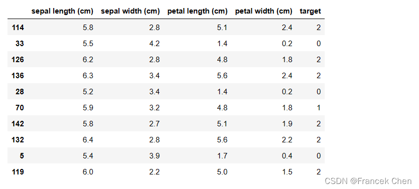
在这里插入图片描述
(二)进行z-score标准化处理
为减小不同特征/属性的量纲差距,下面的代码进行了z-score标准化处理。
from sklearn.preprocessing import StandardScaler
ss=StandardScaler()
new_data=ss.fit_transform(iris.data)
new_df=pd.DataFrame(new_data,columns=iris.feature_names)
#提取每个样本的真实类别标签
new_df['target']=iris.target
new_df.sample(10)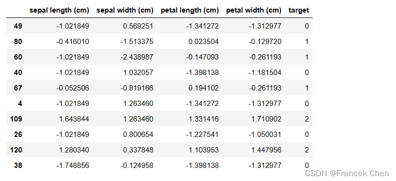
(三)划分训练集和测试集
下面的train_test_split函数将把全部150个样本划分成训练集和测试集,其中测试集占30% (对应于test_size=0.3)。划分时使用了stratify参数进行分层采样 (参考:https://zhuanlan.zhihu.com/p/49991313) ,这样可以保证每个类别的训练样本都是35个。
from sklearn.model_selection import train_test_split

X_train,X_test,y_train,y_test=train_test_split(new_df.iloc[:,0:4],new_df['target'],stratify=new_df['target'],random_state=33,test_size=0.3)
print(y_train.value_counts())
如果不使用stratify参数进行分层采样,有可能使得不同类别的训练样本数量不同,进而影响分类准确性。下面的划分没有使用分层采样,可以发现出现了样本不平衡现象,这会影响后面的分类效果 (去掉注释后可以对比分析)。
#X_train,X_test,y_train,y_test=train_test_split(new_df.iloc[:,0:4],new_df['target'],random_state=33,test_size=0.3)
#print(y_train.value_counts())
(四)进行类别预测和模型性能评估
#https://scikit-learn.org/stable/modules/classes.html#module-sklearn.neighbors

from sklearn.neighbors import KNeighborsClassifier

#下面的语句创建kNN分类估计器,这里指定超参数k等于9,即为了分类,需要找到测试样本的9个近邻去投票
neigh = KNeighborsClassifier(n_neighbors=9)  #n_neighbors默认值是5
#下面的语句进行数据拟合(类似于模型学习),对kNN分类器而言就是构建一颗kd_tree
neigh.fit(X_train,y_train)
#下面的语句进行测试样本的类别预测,对kNN分类器而言就是在kd_tree上找到k个近邻并投票确定测试样本的类别
y_pred=neigh.predict(X_test)#下面的代码用于查看分类性能:
#注意:多分类问题可以使用accuracy_score查看分类的准确性
ACC = metrics.accuracy_score(y_test,y_pred)
print("分类的准确率:",ACC)
#注意:对于多分类问题,却无法使用precision_score/recall_score/f1_score函数
#precision=metrics.precision_score(y_test,y_pred)
#print("分类的查准率:",precision)
#对于多分类问题,却可以使用classification_report函数查看相关性能指标
print("分类性能报告:")
print(classification_report(y_test,y_pred))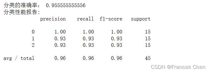
(五)利用网格搜索来优化分类模型的性能
为了找到可能更好的超参数k提升分类的性能,下面的代码演示了交叉验证配合网格搜索。
超参数说明:模型参数 (如果有的话,例如SVM中分离超平面的法向量w和截距b) 是通过fit方法从数据中学习到的,而超参数则是人工配置的,因而创建模型对象时指定的参数是超参数。
为了评估不同超参数组合配置下的模型性能,可以采用网格搜索的方法,并且常常与训练数据集的交叉验证进行搭配。网格搜索的目的是为了优化超参数配置,交叉验证的目的是为了更准确的评估特定超参数配置下的模型性能的可信度,两者作用不同。
关于交叉验证,可以参考: https://www.cnblogs.com/qiu-hua/p/14904992.html https://www.ngui.cc/el/1515667.html?action=onClick
from sklearn.model_selection import GridSearchCV,KFold
from sklearn.neighbors import KNeighborsClassifier
from sklearn.metrics import classification_report

#下面的代码指定了网格搜索的范围,即把从3到9范围内的整数一个个尝试作为超参数k的取值
params_knn={'n_neighbors':range(3,16,1)}
#下面的代码指定进行3折交叉验证,交叉验证的好处(可以自行百度):
#充分利用所有数据、更好地评估模型稳定性、有利于超参数调优、防止过拟合等
kf=KFold(n_splits=3,shuffle=False)

#下面的语句创建kNN分类估计器,创建时所有参数使用默认值
neigh = KNeighborsClassifier()
#下面的语句创建网格搜索估计器,并依次指定分类算法、超参数k的取值范围、交叉验证的设置
grid_search_knn=GridSearchCV(neigh,params_knn,cv=kf)
#下面的语句用创建网格搜索估计器进行训练数据的拟合(类似于模型学习)
grid_search_knn.fit(X_train,y_train)
#下面的语句用拟合好的网格搜索估计器(类似于学习到的模型)进行测试集中所有样本的分类预测
grid_search_y_pred=grid_search_knn.predict(X_test)
#下面的代码用于分类的性能评价
print("分类准确率:",grid_search_knn.score(X_test,y_test))
print("网格搜索得到的最佳超参数:",grid_search_knn.best_params_)
print("输出分类性能报告:")
print(classification_report(y_test,grid_search_y_pred))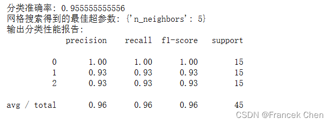
本文参与 腾讯云自媒体同步曝光计划,分享自作者个人站点/博客。
原始发表:2025-01-22,如有侵权请联系 cloudcommunity@tencent.com 删除
评论
登录后参与评论
推荐阅读
目录
腾讯云开发者

Copyright © 2013 - 2026 Tencent Cloud. All Rights Reserved. 腾讯云 版权所有
深圳市腾讯计算机系统有限公司 ICP备案/许可证号:粤B2-20090059 ![]() 粤公网安备44030502008569号
粤公网安备44030502008569号
腾讯云计算(北京)有限责任公司 京ICP证150476号 | 京ICP备11018762号