知识积累---整合细胞形态和空间转录组学深入分析肿瘤生态系统
原创
知识积累---整合细胞形态和空间转录组学深入分析肿瘤生态系统
原创
追风少年i
发布于 2024-08-25 18:06:39
发布于 2024-08-25 18:06:39
作者,Evil Genius
大家科研不要把自己逼得太紧,适当放松是为了更好的工作,比如最近很好的悟空,3个人凑钱买了一份玩一玩,第一关都过不去。
今日参考文献,
虽然作者是中国人,但却是美国的课题组,

我早已工作了,分享了很多的分析方法,但是基本不可能有机会参与原创性的工作了,大家基本上常用的软件,比如Seurat、cellchat等等,都是在美国人的中国人开发的,说明了只要有好的环境,国人的才智简直无可匹敌。
分析目标,绘制癌细胞和TME成分,对细胞类型和状态进行分层,并分析细胞共定位。
知识背景
- 基于下一代测序(NGS)的平台,如Visium、GeoMx、Slide-Seq。基于杂交的方法,如MERFISH、seqFISH和CosMx。基于NGS的ST方法覆盖了整个转录组,但不是单细胞分辨率,而基于原位杂交的方法提供了优越的空间分辨率,但仅限于基因组的一小部分,限制了它们在基于发现的研究中的潜力(不过5000+探针还是可以的)。
- 通过结合空间基因表达、组织组织学和癌症和TME细胞的先验知识,系统地分析癌细胞和TME细胞。
METI 分析框架
- 重点关注从正常细胞到癌前细胞再到恶性细胞的进展,同时也检查每个组织切片内的淋巴细胞。
- METI的目标是精确识别各种细胞类型及其在TME中的各自状态。
模块1,METI识别正常细胞和癌前细胞. 模块2,METI识别肿瘤细胞富集区并表征其细胞状态的异质性 模块3, T细胞的空间定位 模块4,中识别其他免疫细胞,包括中性粒细胞、B细胞、浆细胞和巨噬细胞。 模块5、成纤维细胞的分析
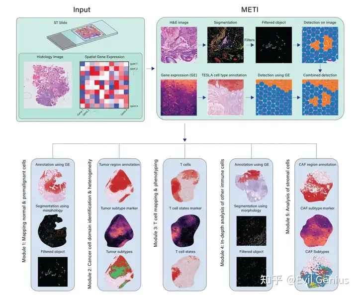
模块一、绘制正常细胞和癌前细胞
分析思路:病理学家标注 + 正常细胞的形态学形状 + 基因表达数据
- 这种检测不能通过流行的空间聚类方法单独实现
模块二、癌细胞结构域和异质性的鉴定
大多数实体瘤起源于上皮细胞,被称为癌,包括胃癌、肺癌、膀胱癌、乳腺癌、前列腺癌和结肠癌,而其他一些实体瘤起源于其他类型的组织,包括肉瘤和黑色素瘤。无论其细胞来源如何,了解恶性细胞的分子特征和细胞异质性对于揭示肿瘤生长、侵袭、转移和治疗反应的机制至关重要。定量生物组织内细胞的空间分布和密度对于各种应用至关重要,特别是在病理学和肿瘤学领域。虽然基因表达提供了一个molecular lens,但相关的H&E图像可以用来测量空间细胞分布和密度。与模块1一样,METI接下来进行肿瘤细胞核分割,生成三维肿瘤细胞密度图,直观地描绘了癌细胞的空间分布和密度。该功能用于传达感兴趣的细胞类型的空间分布、密度和模式。
模块三、T细胞定位和表型
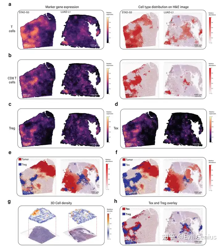
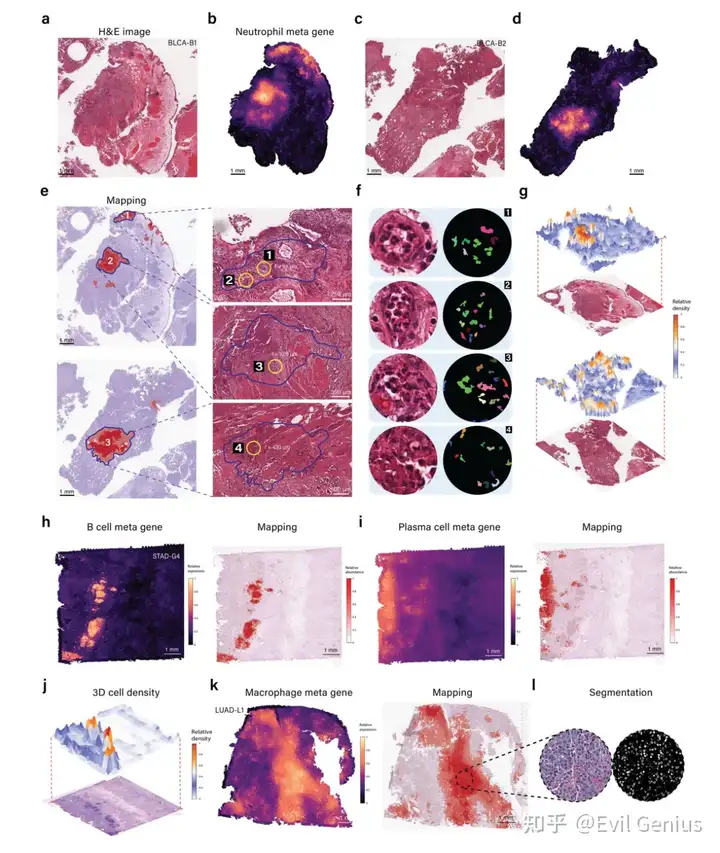
模块4、深入分析其他免疫细胞,这其中就包括了单细胞难以捕获到的中性粒细胞。
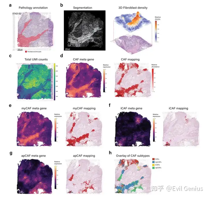
模块5、成纤维细胞的分析
示例代码在 https://github.com/Flashiness/METI。
我们简单看一下,注意如果运用到自己的课题还是需要认真思考的。
##pip install METIforST
#Note: you need to make sure that the pip is for python3,or you can install METI by
##python3 -m pip install METIforST==0.2

import torch
import csv,re, time
import pickle
import random
import warnings
warnings.filterwarnings('ignore')
import pandas as pd
import numpy as np
from scipy import stats
from scipy.sparse import issparse
import scanpy as sc
import matplotlib.colors as clr
import matplotlib.pyplot as plt
import cv2
import TESLA as tesla
from IPython.display import Image
import scipy.sparse
import scanpy as sc
import pandas as pd
import matplotlib.pyplot as plt
import seaborn as sns
from scanpy import read_10x_h5
import PIL
from PIL import Image as IMAGE
import os
import METI as meti
import tifffile
os.environ['KMP_DUPLICATE_LIB_OK']='True'
读取数据
adata=sc.read_visium("/tutorial/data/Spaceranger/")
spatial=pd.read_csv("/tutorial/data/Spaceranger/tissue_positions_list.csv",sep=",",header=None,na_filter=False,index_col=0)

adata.var_names_make_unique()
adata.var["mt"] = adata.var_names.str.startswith("MT-")
sc.pp.calculate_qc_metrics(adata, qc_vars=["mt"], inplace=True)

plt.rcParams["figure.figsize"] = (8, 8)
sc.pl.spatial(adata, img_key="hires", color=["total_counts", "n_genes_by_counts"], size = 1.5, save = 'UMI_count.png')
转换数据

#================== 3. Read in data ==================#
#Read original 10x_h5 data and save it to h5ad
from scanpy import read_10x_h5
adata = read_10x_h5("../tutorial/data/filtered_feature_bc_matrix.h5")
spatial=pd.read_csv("../tutorial/data/tissue_positions_list.csv",sep=",",header=None,na_filter=False,index_col=0)
adata.obs["x1"]=spatial[1]
adata.obs["x2"]=spatial[2]
adata.obs["x3"]=spatial[3]
adata.obs["x4"]=spatial[4]
adata.obs["x5"]=spatial[5]
adata.obs["array_x"]=adata.obs["x2"]
adata.obs["array_y"]=adata.obs["x3"]
adata.obs["pixel_x"]=adata.obs["x4"]
adata.obs["pixel_y"]=adata.obs["x5"]
#Select captured samples
adata=adata[adata.obs["x1"]==1]
adata.var_names=[i.upper() for i in list(adata.var_names)]
adata.var["genename"]=adata.var.index.astype("str")
adata.write_h5ad("../tutorial/data/1957495_data.h5ad")
#Read in gene expression and spatial location
counts=sc.read("../tutorial/data/1957495_data.h5ad")
#Read in hitology image
PIL.Image.MAX_IMAGE_PIXELS = None
img = IMAGE.open(r"../tutorial/data/histology.tif")
img = np.array(img)
#if your image has 4 dimensions, only keep first 3 dims
img=img[...,:3]
resize_factor=1000/np.min(img.shape[0:2])
resize_width=int(img.shape[1]*resize_factor)
resize_height=int(img.shape[0]*resize_factor)
counts.var.index=[i.upper() for i in counts.var.index]
counts.var_names_make_unique()
counts.raw=counts
sc.pp.log1p(counts) # impute on log scale
if issparse(counts.X):counts.X=counts.X.A
###Contour detection
# Detect contour using cv2
cnt=tesla.cv2_detect_contour(img, apertureSize=5,L2gradient = True)
binary=np.zeros((img.shape[0:2]), dtype=np.uint8)
cv2.drawContours(binary, [cnt], -1, (1), thickness=-1)
#Enlarged filter
cnt_enlarged = tesla.scale_contour(cnt, 1.05)
binary_enlarged = np.zeros(img.shape[0:2])
cv2.drawContours(binary_enlarged, [cnt_enlarged], -1, (1), thickness=-1)
img_new = img.copy()
cv2.drawContours(img_new, [cnt], -1, (255), thickness=20)
img_new=cv2.resize(img_new, ((resize_width, resize_height)))
cv2.imwrite('../tutorial/data/cnt_1957495.jpg', img_new)
Image(filename='../tutorial/data/cnt_1957495.jpg')
####Gene expression enhancement
#Set size of superpixel
res=40
# Note, if the numer of superpixels is too large and take too long, you can increase the res to 100
enhanced_exp_adata=tesla.imputation(img=img, raw=counts, cnt=cnt, genes=counts.var.index.tolist(), shape="None", res=res, s=1, k=2, num_nbs=10)
enhanced_exp_adata.write_h5ad("../tutorial/data/enhanced_exp.h5ad")
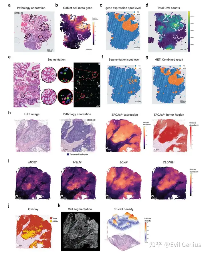
####Goblet marker gene expression
#================ determine if markers are in ===============#
enhanced_exp_adata=sc.read("..tutorial/data/enhanced_exp.h5ad")
markers = ["MS4A10", "MGAM", "CYP4F2", "XPNPEP2", "SLC5A9", "SLC13A2", "SLC28A1", "MEP1A", "ABCG2", "ACE2"]
for i in range(len(markers)):
if markers[i] in enhanced_exp_adata.var.index: print("yes")
else: print(markers[i])
save_dir="..tutorial/data/Goblet/"
if not os.path.exists(save_dir):os.mkdir(save_dir)
#================ Plot gene expression image ===============#
markers = ["MS4A10", "MGAM", "CYP4F2", "XPNPEP2", "SLC5A9", "SLC13A2", "SLC28A1", "MEP1A", "ABCG2", "ACE2"]
for i in range(len(markers)):
cnt_color = clr.LinearSegmentedColormap.from_list('magma', ["#000003", "#3b0f6f", "#8c2980", "#f66e5b", "#fd9f6c", "#fbfcbf"], N=256)
g=markers[i]
enhanced_exp_adata.obs[g]=enhanced_exp_adata.X[:,enhanced_exp_adata.var.index==g]
fig=sc.pl.scatter(enhanced_exp_adata,alpha=1,x="y",y="x",color=g,color_map=cnt_color,show=False,size=10)
fig.set_aspect('equal', 'box')
fig.invert_yaxis()
plt.gcf().set_dpi(600)
fig.figure.show()
plt.savefig(save_dir + str(markers[i]) + ".png", dpi=600)
plt.close()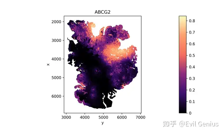
#================ Plot meta gene expression image ===============#
enhanced_exp_adata=sc.read("/Users/jjiang6/Desktop/UTH/MDA GRA/Spatial transcriptome/Cell Segmentation/With Jian Hu/S1_54078/TESLA/enhanced_exp.h5ad")
genes =   ["MS4A10", "MGAM", "CYP4F2", "XPNPEP2", "SLC5A9", "SLC13A2", "SLC28A1", "MEP1A", "ABCG2", "ACE2"]

sudo_adata = meti.meta_gene_plot(img=img,
                                binary=binary,
                                sudo_adata=enhanced_exp_adata,
                                genes=genes,
                                resize_factor=resize_factor,
                                target_size="small")

cnt_color = clr.LinearSegmentedColormap.from_list('magma', ["#000003",  "#3b0f6f",  "#8c2980",   "#f66e5b", "#fd9f6c", "#fbfcbf"], N=256)
fig=sc.pl.scatter(sudo_adata,alpha=1,x="y",y="x",color='meta',color_map=cnt_color,show=False,size=5)
fig.set_aspect('equal', 'box')
fig.invert_yaxis()
plt.gcf().set_dpi(600)
fig.figure.show()

plt.savefig(save_dir + "Goblet_meta.png", dpi=600)
plt.close()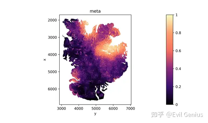
Region annotation
genes=["MS4A10", "MGAM", "CYP4F2", "XPNPEP2", "SLC5A9", "SLC13A2", "SLC28A1", "MEP1A", "ABCG2", "ACE2"]
genes=list(set([i for i in genes if i in enhanced_exp_adata.var.index ]))
#target_size can be set to "small" or "large".
pred_refined, target_clusters, c_m=meti.annotation(img=img,
                                                    binary=binary,
                                                    sudo_adata=enhanced_exp_adata,
                                                    genes=genes,
                                                    resize_factor=resize_factor,
                                                    num_required=1,
                                                    target_size="small")
#Plot
ret_img=tesla.visualize_annotation(img=img,
                              binary=binary,
                              resize_factor=resize_factor,
                              pred_refined=pred_refined,
                              target_clusters=target_clusters,
                              c_m=c_m)

cv2.imwrite(save_dir + 'IME.jpg', ret_img)
Image(filename=save_dir + 'IME.jpg')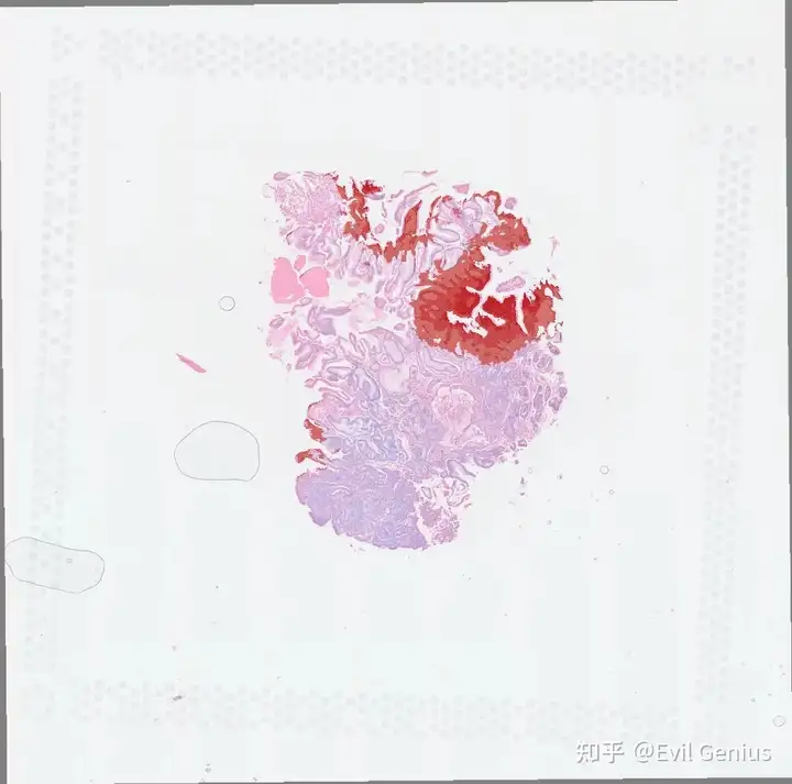
#=====================================Convert to spot level============================================#
adata.obs["color"]=extract_color(x_pixel=(np.array(adata.obs["pixel_x"])*resize_factor).astype(np.int64),
                                 y_pixel=(np.array(adata.obs["pixel_y"])*resize_factor).astype(np.int64), image=ret_img, beta=25)

type = []
for each in adata.obs["color"]:
    if each < adata.obs["color"].quantile(0.2):
        r = "yes"
        type.append(r)
    else:
        r = "no"
        type.append(r)

adata.obs['Goblet_GE'] = type

fig, ax = plt.subplots(figsize=(10, 10))  # Adjust the size as needed
ax.imshow(img)
ax.set_axis_off()
sc.pl.scatter(adata, x='pixel_y', y='pixel_x', color='Goblet_GE', ax=ax, size = 150, title='Goblet GE Spot Annotations')
# Save the figure
plt.savefig('./sample_results/Goblet_spot_GE.png', dpi=300, bbox_inches='tight')
图像分割Segmentation
plot_dir="/rsrch4/home/genomic_med/jjiang6/Project1/S1_54078/Segmentation/NC_review_Goblet_seg/"
save_dir=plot_dir+"/seg_results"
adata= sc.read("/rsrch4/home/genomic_med/jjiang6/Project1/S1_54078/TESLA/54078_data.h5ad")

img_path = '/rsrch4/home/genomic_med/jjiang6/Project1/S1_54078/1415785-6 Bx2.tif'
img = tiff.imread(img_path)
d0, d1= img.shape[0], img.shape[1]

#=====================================Split into patched=====================================================
patch_size=400
patches=patch_split_for_ST(img=img, patch_size=patch_size, spot_info=adata.obs, x_name="pixel_x", y_name="pixel_y")
patch_info=adata.obs

# save results
pickle.dump(patches, open(plot_dir + 'patches.pkl', 'wb'))
#=================================Image Segmentation===================================
meti.Segment_Patches(patches, save_dir=save_dir,n_clusters=10)

#=================================Get masks=================================#
pred_file_locs=[save_dir+"/patch"+str(j)+"_pred.npy" for j in range(patch_info.shape[0])]
dic_list=meti.get_color_dic(patches, seg_dir=save_dir)
masks_index=meti.Match_Masks(dic_list, num_mask_each=5, mapping_threshold1=30, mapping_threshold2=60)

masks=meti.Extract_Masks(masks_index, pred_file_locs, patch_size)

combined_masks=meti.Combine_Masks(masks, patch_info, d0, d1)

#=================================Plot masks=================================#
plot_dir = '../tutorial/data/seg_results/mask'

for i in range(masks.shape[0]): #Each mask
    print("Plotting mask ", str(i))
    ret=(combined_masks[i]*255)
    cv2.imwrite(plot_dir+'/mask'+str(i)+'.png', ret.astype(np.uint8))

#=================================Choose one mask to detect cells/nucleis=================================#
channel=1
converted_image = combined_masks[1].astype(np.uint8)
ret, labels = cv2.connectedComponents(converted_image)
features=meti.Extract_CC_Features_each_CC(labels)

num_labels = labels.max()
height, width = labels.shape

colors = np.random.randint(0, 255, size=(num_labels + 1, 3), dtype=np.uint8)
colors[0] = [0, 0, 0]
colored_mask = np.zeros((height, width, 3), dtype=np.uint8)
colored_mask = colors[labels]

# save the colored nucleis channel
cv2.imwrite('/rsrch4/home/genomic_med/jjiang6/Project1/S1_54078/Segmentation/NC_review_Goblet_seg/seg_results/goblet.png', colored_mask)
# save nucleis label
np.save('/rsrch4/home/genomic_med/jjiang6/Project1/S1_54078/Segmentation/NC_review_Goblet_seg/seg_results/labels.npy', labels)
# save nucleis features, including, area, length, width
features.to_csv('/rsrch4/home/genomic_med/jjiang6/Project1/S1_54078/Segmentation/NC_review_Goblet_seg/seg_results/features.csv', index=False)

#=================================filter out goblet cells=================================#
plot_dir="../tutorial/data/seg_results/mask"
if not os.path.exists(plot_dir):os.mkdir(plot_dir)

labels=np.load(plot_dir+"labels.npy")

#Filter - different cell type needs to apply different parameter values
features=pd.read_csv(plot_dir+"features.csv", header=0, index_col=0)
features['mm_ratio'] = features['major_axis_length']/features['minor_axis_length']
features_sub=features[(features["area"]>120) &
                      (features["area"]<1500) &
                      (features["solidity"]>0.85) &
                      (features["mm_ratio"]<2)]
index=features_sub.index.tolist()
labels_filtered=labels*np.isin(labels, index)

np.save(plot_dir+"nuclei_filtered.npy", labels_filtered)

num_labels = labels_filtered.max()
height, width = labels_filtered.shape

colors = np.random.randint(0, 255, size=(num_labels + 1, 3), dtype=np.uint8)
colors[0] = [0, 0, 0]
colored_mask = np.zeros((height, width, 3), dtype=np.uint8)
colored_mask = colors[labels_filtered]

cv2.imwrite(plot_dir+'/goblet_filtered.png', colored_mask)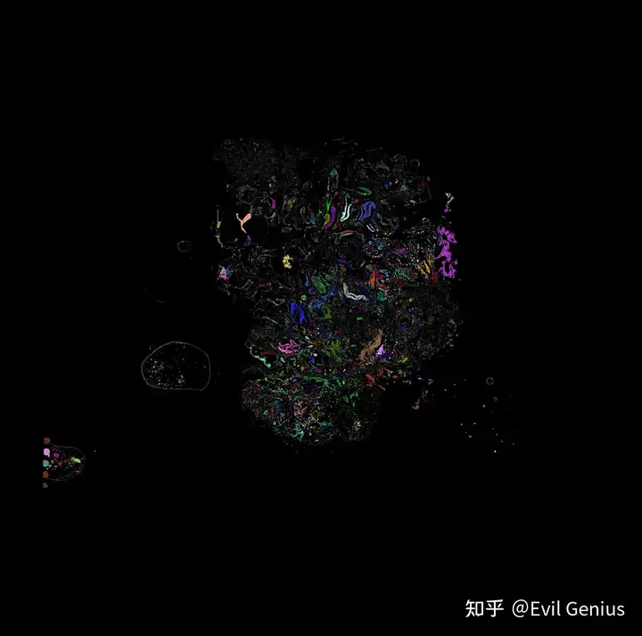
nuclei segmentation
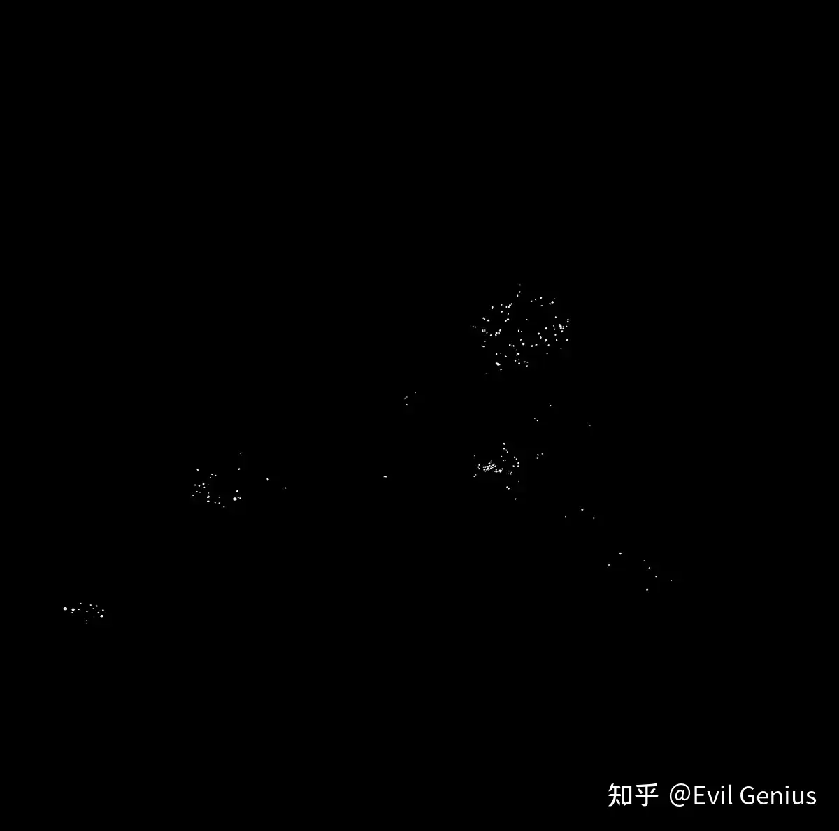
goblet segmentation
#=====================================Convert to spot level============================================#
plot_dir="./tutorial/sample_results/"
img_seg = np.load(plot_dir+'nuclei_filtered_white.npy')

adata.obs["color"]=meti.extract_color(x_pixel=(np.array(adata.obs["pixel_x"])).astype(np.int64),
                    y_pixel=(np.array(adata.obs["pixel_y"])).astype(np.int64), image=img_seg, beta=49)

type = []
for each in adata.obs["color"]:
    if each > 0:
        r = "yes"
        type.append(r)
    else:
        r = "no"
        type.append(r)

adata.obs['Goblet_seg'] = type

fig, ax = plt.subplots(figsize=(10, 10))
ax.imshow(img)
ax.set_axis_off()
sc.pl.scatter(adata, x='pixel_y', y='pixel_x', color='Goblet_seg', ax=ax, size = 150, title='Goblet Segmentation Spot Annotations')
# Save the figure
plt.savefig(plot_dir+'Goblet_spot_seg.png', format='png', dpi=300, bbox_inches='tight')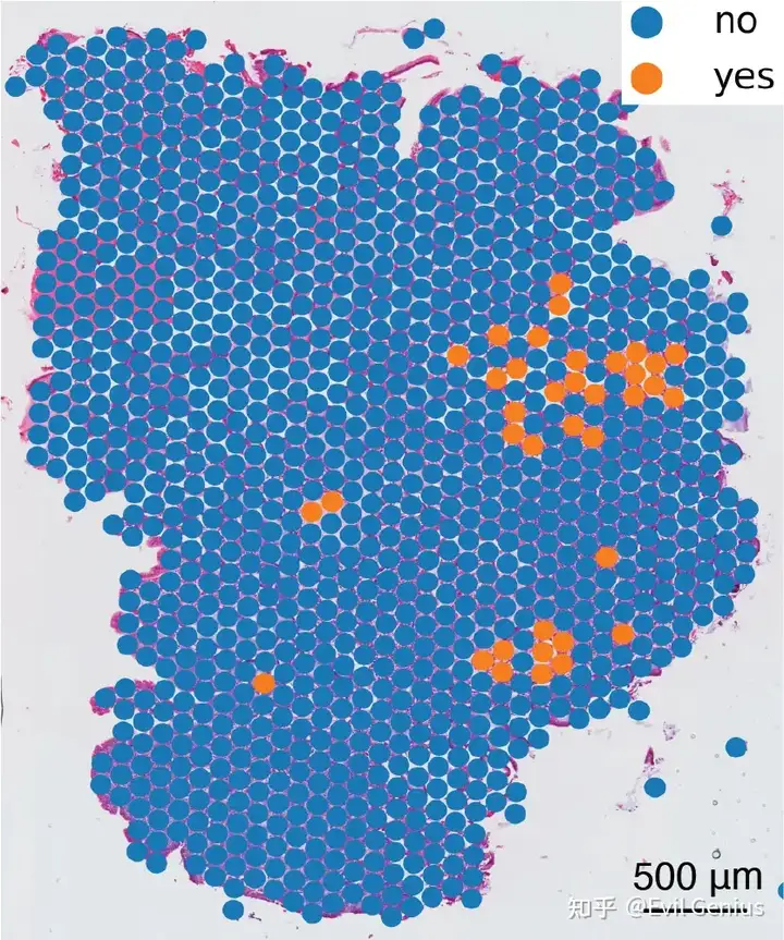
Integrarion of gene expression result with segmentation result
adata.obs['Goblet_combined'] = np.where((adata.obs['Goblet_seg'] == 'yes') | (adata.obs['Goblet_GE'] == 'yes'), 'yes', 'no')

fig, ax = plt.subplots(figsize=(10, 10))
ax.imshow(img)
ax.set_axis_off()
sc.pl.scatter(adata, x='pixel_y', y='pixel_x', color='Goblet_combined', ax=ax, size = 150,title='Goblet Combined Spot Annotations')
# Save the figure
plt.savefig(plot_dir+'Goblet_spot_combined.png', format='png', dpi=300, bbox_inches='tight')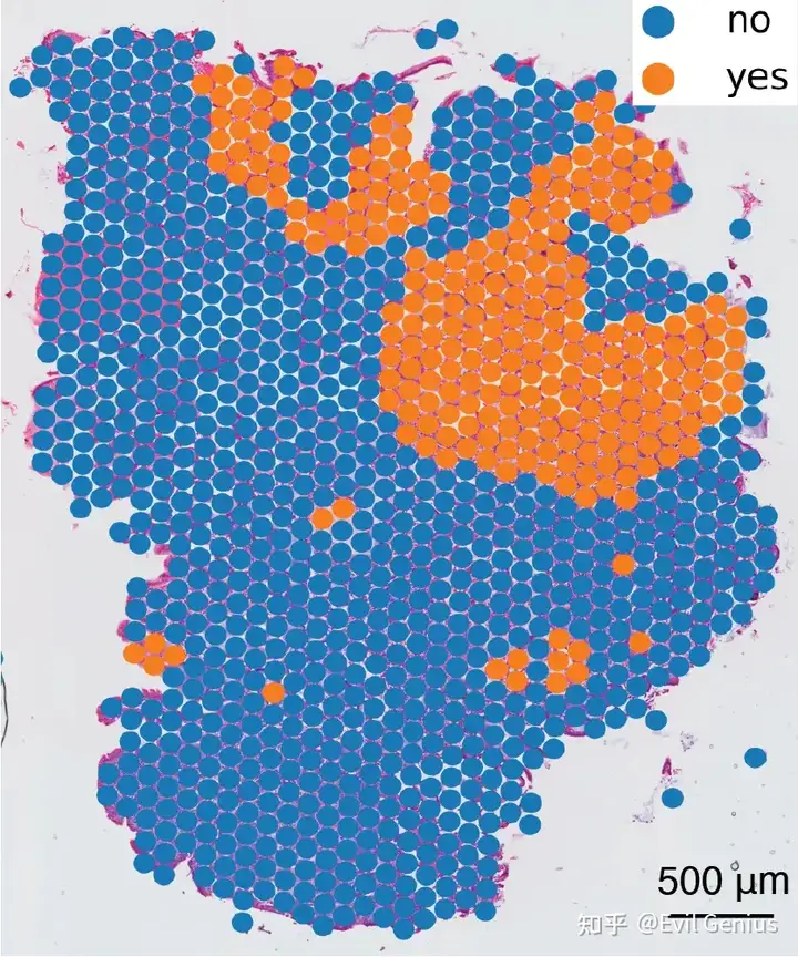
goblet combined result spot level
生活很好,有你更好
原创声明:本文系作者授权腾讯云开发者社区发表,未经许可,不得转载。
如有侵权,请联系 cloudcommunity@tencent.com 删除。
原创声明:本文系作者授权腾讯云开发者社区发表,未经许可,不得转载。
如有侵权,请联系 cloudcommunity@tencent.com 删除。
评论
登录后参与评论
推荐阅读
目录
腾讯云开发者

Copyright © 2013 - 2026 Tencent Cloud. All Rights Reserved. 腾讯云 版权所有
深圳市腾讯计算机系统有限公司 ICP备案/许可证号:粤B2-20090059 ![]() 粤公网安备44030502008569号
粤公网安备44030502008569号
腾讯云计算(北京)有限责任公司 京ICP证150476号 | 京ICP备11018762号