GEO数据库中芯片数据分析思路
原创

GEO数据库中芯片数据分析思路
- 找数据,找到GSE编号
- 下载数据:表达矩阵 临床信息,分组信息 GPL编号 注:GEO数据库中array就是芯片数据,GSE开头为数据集编号,GPL平台编号,GSM样本名。
- 数据探索:分组之间是否有差异,PCA,热图
- 差异分析及可视化:p值,logFC 火山图,热图
- 富集分析KEGG,GO
数据下载
#实战代码有很多注意事项, 请不要不听课直接跑代码。
rm(list = ls())
library(GEOquery)
#先去网页确定是否是表达芯片数据,不是的话不能用本流程。
gse_number = "GSE42872"
eSet <- getGEO(gse_number, destdir = '.', getGPL = F)
##下载并读取数据,本地有的话会识别,本地不完整的话要删掉
##destdir = '.'下载在当前目录, getGPL = F不下载注释文件。
class(eSet)## [1] "list"length(eSet)## [1] 1eSet = eSet[[1]]
#(1)提取表达矩阵exp
exp <- exprs(eSet)
dim(exp)## [1] 33297 6exp[1:4,1:4]## GSM1052615 GSM1052616 GSM1052617 GSM1052618
## 7892501 7.24559 6.80686 7.73301 6.18961
## 7892502 6.82711 6.70157 7.02471 6.20493
## 7892503 4.39977 4.50781 4.88250 4.36295
## 7892504 9.48025 9.67952 9.63074 9.69200#检查矩阵是否正常,如果是空的就会报错,空的和有负值的、有异常值的矩阵需要处理原始数据。
#如果表达矩阵为空,大多数是转录组数据,不能用这个流程(后面另讲)。
#自行判断是否需要log
#exp = log2(exp+1)
boxplot(exp)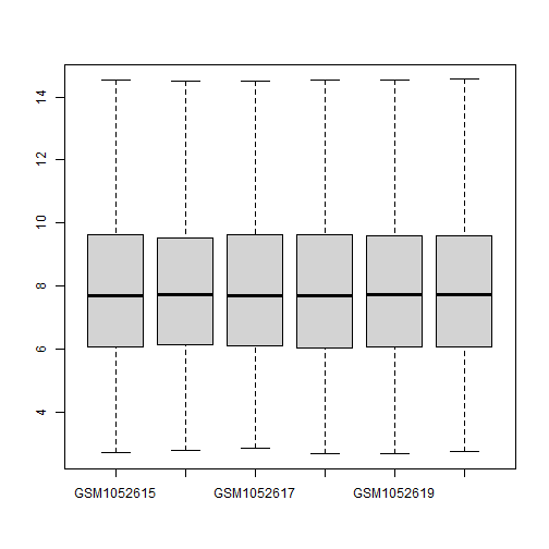
#(2)提取临床信息
pd <- pData(eSet)
#(3)让exp列名与pd的行名顺序完全一致
p = identical(rownames(pd),colnames(exp));p## [1] TRUEif(!p) exp = exp[,match(rownames(pd),colnames(exp))]
# 分组信息来自临床信息,分组信息需要与表达矩阵列名一一对应,
# 临床信息需要和表达矩阵列一一对应
#(4)提取芯片平台编号
gpl_number <- eSet@annotation;gpl_number## [1] "GPL6244"save(gse_number,pd,exp,gpl_number,file = "step1output.Rdata")取过log的数据大小在0-15之间,也可以通过箱线图查看。
- 正常表达矩阵数值范围在0-20之间。
- 箱线图中位数线相对平齐,标准化后非常齐,因为样本绝大多数是没有差异的。
- 如果有的样本中位数和别的不一样,就是异常样本,要删除异常样本,或者标准化。
# Group(实验分组)和ids(探针注释)
rm(list = ls())
load(file = "step1output.Rdata")
library(stringr)
# 标准流程代码是二分组,多分组数据的分析后面另讲
# 生成Group向量的三种常规方法,三选一,选谁就把第几个逻辑值写成T,另外两个为F。如果三种办法都不适用,可以继续往后写else if
if(F){
# 1.Group----
# 第一种方法,有现成的可以用来分组的列
Group = pd$`disease state:ch1`
}else if(F){
# 第二种方法,自己生成
Group = c(rep("RA",times=13),
rep("control",times=9))
Group = rep(c("RA","control"),times = c(13,9))
}else if(T){
# 第三种方法,使用字符串处理的函数获取分组
Group=ifelse(str_detect(pd$title,"Control"),
"control",
"RA")##匹配关键词
}
# 需要把Group转换成因子,并设置参考水平,指定levels,对照组在前,处理组在后
Group = factor(Group,levels = c("control","RA"))
Group## [1] control control control RA RA RA
## Levels: control RA##factor因子有水平,即取值。
##levels水平有顺序,第一个位置是领头羊,是参考水平。
##levels水平可以默认生成,也可以自行指定。
##参考水平的用处:差异分析时自动作为对照组。2.探针注释的获取
注释来源: 1.Biocoductor的注释包
- GPL的表格文件解析
- 官网下载对应产品的注释表格
- 自主注释
AnnoProbe是曾建明老师2020年开发的一款用于下载GEO数据集并注释的R包,收录在tinyarray里。 idmap##根据所给的GPL号,返回探针的注释 geoChina##根据所给的GSE号,下载对应的表达矩阵 annoGene##根据gencode中的GTF文件注释基因ID
#捷径
library(tinyarray)
find_anno(gpl_number) #打出找注释的代码
ids <- AnnoProbe::idmap('GPL6244')
##是曾建明老师2020年开发的一款用于下载GEO数据集并注释的R包
?idmap##根据所给的GPL号,返回探针的注释
?geoChina##根据所给的GSE号,下载对应的表达矩阵
?annoGene##根据gencode中的GTF文件注释基因ID
#四种方法,方法1里找不到就从方法2找,以此类推。
#方法1 BioconductorR包(最常用)
gpl_number ## [1] "GPL6244"#在该网站找到芯片平台编号对应的物种和探针的注释信息R包
##http://www.bio-info-trainee.com/1399.html
if(!require(hugene10sttranscriptcluster.db))BiocManager::install("hugene10sttranscriptcluster.db")
library(hugene10sttranscriptcluster.db)
ls("package:hugene10sttranscriptcluster.db")## [1] "hugene10sttranscriptcluster" "hugene10sttranscriptcluster.db"
## [3] "hugene10sttranscriptcluster_dbconn" "hugene10sttranscriptcluster_dbfile"
## [5] "hugene10sttranscriptcluster_dbInfo" "hugene10sttranscriptcluster_dbschema"
## [7] "hugene10sttranscriptclusterACCNUM" "hugene10sttranscriptclusterALIAS2PROBE"
## [9] "hugene10sttranscriptclusterCHR" "hugene10sttranscriptclusterCHRLENGTHS"
## [11] "hugene10sttranscriptclusterCHRLOC" "hugene10sttranscriptclusterCHRLOCEND"
## [13] "hugene10sttranscriptclusterENSEMBL" "hugene10sttranscriptclusterENSEMBL2PROBE"
## [15] "hugene10sttranscriptclusterENTREZID" "hugene10sttranscriptclusterENZYME"
## [17] "hugene10sttranscriptclusterENZYME2PROBE" "hugene10sttranscriptclusterGENENAME"
## [19] "hugene10sttranscriptclusterGO" "hugene10sttranscriptclusterGO2ALLPROBES"
## [21] "hugene10sttranscriptclusterGO2PROBE" "hugene10sttranscriptclusterMAP"
## [23] "hugene10sttranscriptclusterMAPCOUNTS" "hugene10sttranscriptclusterOMIM"
## [25] "hugene10sttranscriptclusterORGANISM" "hugene10sttranscriptclusterORGPKG"
## [27] "hugene10sttranscriptclusterPATH" "hugene10sttranscriptclusterPATH2PROBE"
## [29] "hugene10sttranscriptclusterPFAM" "hugene10sttranscriptclusterPMID"
## [31] "hugene10sttranscriptclusterPMID2PROBE" "hugene10sttranscriptclusterPROSITE"
## [33] "hugene10sttranscriptclusterREFSEQ" "hugene10sttranscriptclusterSYMBOL"
## [35] "hugene10sttranscriptclusterUNIPROT"ids <- toTable(hugene10sttranscriptclusterSYMBOL)##以data.frame格式提取数据
head(ids)## probe_id symbol
## 1 7896746 MTND1P23
## 2 7896754 SEPTIN7P13
## 3 7896759 LINC01128
## 4 7896761 SAMD11
## 5 7896779 KLHL17
## 6 7896798 PLEKHN1# 方法2 读取GPL网页的表格文件,按列取子集
##https://www.ncbi.nlm.nih.gov/geo/query/acc.cgi?acc=GPL570
if(F){
#注:表格读取参数、文件列名不统一,活学活用,有的表格里没有symbol列,也有的GPL平台没有提供注释表格
b = read.delim("GPL570-55999.txt",
check.names = F,
comment.char = "#")
colnames(b)
ids2 = b[,c("ID","Gene Symbol")]
colnames(ids2) = c("probe_id","symbol")
k1 = ids2$symbol!="";table(k1)
k2 = !str_detect(ids2$symbol,"///");table(k2)
ids2 = ids2[ k1 & k2,]
# ids = ids2
}
# 方法3 官网下载注释文件并读取
##http://www.affymetrix.com/support/technical/byproduct.affx?product=hg-u133-plus
# 方法4 自主注释
#https://mp.weixin.qq.com/s/mrtjpN8yDKUdCSvSUuUwcA
save(exp,Group,ids,gse_number,file = "step2output.Rdata") ##保存数据- PCA图,热图绘制
rm(list = ls())
load(file = "step1output.Rdata")##导入数据
load(file = "step2output.Rdata")
#输入数据:exp和Group
#Principal Component Analysis
#http://www.sthda.com/english/articles/31-principal-component-methods-in-r-practical-guide/112-pca-principal-component-analysis-essentials
# 1.PCA 图----
dat=as.data.frame(t(exp))##将数据转置,处理成PCA接受的数据格式。仅PCA适用,所以要赋值给dat。
library(FactoMineR)
library(factoextra)
dat.pca <- PCA(dat, graph = FALSE)
pca_plot <- fviz_pca_ind(dat.pca,
geom.ind = "point", # show points only (nbut not "text")
col.ind = Group, # color by groups
palette = c("#00AFBB", "#E7B800"),
addEllipses = TRUE, # Concentration ellipses
legend.title = "Groups"
)
pca_plot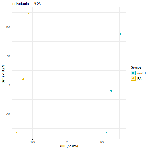
save(pca_plot,file = "pca_plot.Rdata")
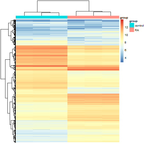
# 2.top 1000 sd 热图----
cg=names(tail(sort(apply(exp,1,sd)),1000))##apply,对exp按行求标准差。
n=exp[cg,]
# 直接画热图,对比不鲜明
library(pheatmap)
annotation_col=data.frame(group=Group)
rownames(annotation_col)=colnames(n) ##写一个分组信息的矩阵
pheatmap(n,
show_colnames =F,
show_rownames = F,
annotation_col=annotation_col
)
# 按行标准化
pheatmap(n,
show_colnames =F,
show_rownames = F,
annotation_col=annotation_col,
scale = "row", ##按行标准化
breaks = seq(-3,3,length.out = 100)##色带范围改变,随机生成100个数
) 
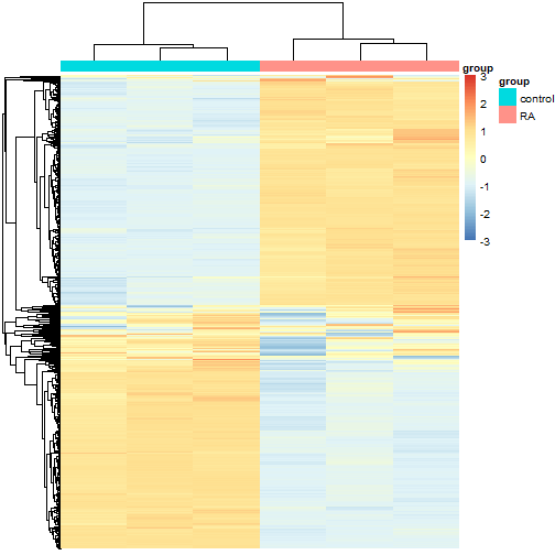
dev.off()## png
## 4limma包做差异分析
rm(list = ls())
load(file = "step2output.Rdata")
#差异分析,用limma包来做
#需要表达矩阵和Group,不需要改
library(limma)
design=model.matrix(~Group)
fit=lmFit(exp,design)
fit=eBayes(fit)
deg=topTable(fit,coef=2,number = Inf)
#为deg数据框添加几列
#1.加probe_id列,把行名变成一列
library(dplyr)
deg <- mutate(deg,probe_id=rownames(deg))
#2.加上探针注释
ids = ids[!duplicated(ids$symbol),]
#其他去重方式在zz.去重方式.R
deg <- inner_join(deg,ids,by="probe_id")
nrow(deg)## [1] 18857#3.加change列,标记上下调基因
logFC_t=1
p_t = 0.05
k1 = (deg$P.Value < p_t)&(deg$logFC < -logFC_t)
k2 = (deg$P.Value < p_t)&(deg$logFC > logFC_t)
deg <- mutate(deg,change = ifelse(k1,"down",ifelse(k2,"up","stable")))
table(deg$change)##
## down stable up
## 489 17782 586#4.加ENTREZID列,用于富集分析(symbol转entrezid,然后inner_join)
library(clusterProfiler)
library(org.Hs.eg.db)
s2e <- bitr(deg$symbol,
fromType = "SYMBOL",
toType = "ENTREZID",
OrgDb = org.Hs.eg.db)#人类
#其他物种http://bioconductor.org/packages/release/BiocViews.html#___OrgDb
deg <- inner_join(deg,s2e,by=c("symbol"="SYMBOL"))
save(Group,deg,logFC_t,p_t,gse_number,file = "step4output.Rdata")火山图,热图
rm(list = ls())
load(file = "step1output.Rdata")
load(file = "step4output.Rdata")
#1.火山图----
library(dplyr)
library(ggplot2)
dat = distinct(deg,symbol,.keep_all = T)
p <- ggplot(data = dat,
aes(x = logFC,
y = -log10(P.Value))) +
geom_point(alpha=0.4, size=3.5,
aes(color=change)) +
scale_color_manual(values=c("blue", "grey","red"))+
geom_vline(xintercept=c(-logFC_t,logFC_t),lty=4,col="black",linewidth=0.8) +
geom_hline(yintercept = -log10(p_t),lty=4,col="black",linewidth=0.8) +
theme_bw()
p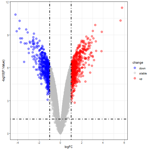
for_label <- dat%>%
filter(symbol %in% c("DUSP6","CD36"))##展示基因名
volcano_plot <- p +
geom_point(size = 3, shape = 1, data = for_label) +
ggrepel::geom_label_repel(
aes(label = symbol),
data = for_label,
color="black"
)
volcano_plot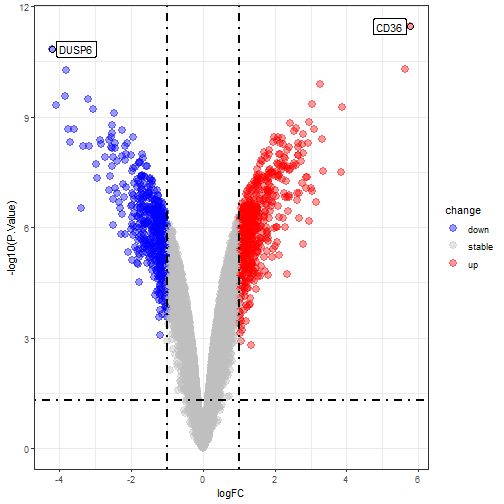
#2.差异基因热图----
load(file = 'step2output.Rdata')
# 表达矩阵行名替换
exp = exp[dat$probe_id,]
rownames(exp) = dat$symbol
if(T){
#取前10上调和前10下调
library(dplyr)
dat2 = dat %>%
filter(change!="stable") %>%
arrange(logFC)
cg = c(head(dat2$symbol,10),
tail(dat2$symbol,10))
}else{
#全部差异基因
cg = dat$symbol[dat$change !="stable"]
length(cg)
}
n=exp[cg,]
dim(n)## [1] 20 6#差异基因热图
library(pheatmap)
annotation_col=data.frame(group=Group)
rownames(annotation_col)=colnames(n)
heatmap_plot <- pheatmap(n,show_colnames =F,
scale = "row",
#cluster_cols = F,
annotation_col=annotation_col,
breaks = seq(-1,1,length.out =100)##色带范围改变,随机生成100个数
)
heatmap_plot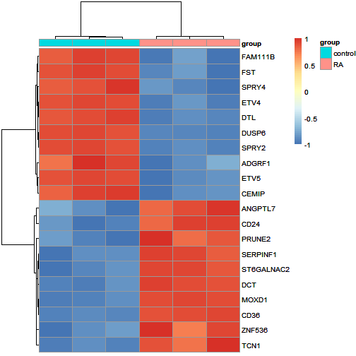
#拼图
library(patchwork)
volcano_plot + heatmap_plot$gtable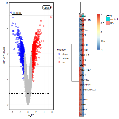
# 3.感兴趣基因的相关性----
library(corrplot)
g = sample(deg$symbol[1:5000],10) # 这里是随机取样,注意换成自己感兴趣的基因
g## [1] "BVES" "RETREG1" "ZBTB2" "ENPP3" "EMC8" "MATN2" "POLE" "MRAS" "DIPK1B"
## [10] "SMAD5"M = cor(t(exp[g,])) ###cor计算相关性。转置后基因变成列,按列做相关性
pheatmap(M)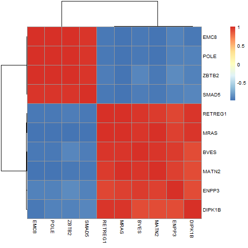
library(paletteer)#配色包
my_color = rev(paletteer_d("RColorBrewer::RdYlBu"))##颜色顺序倒置
my_color = colorRampPalette(my_color)(10)
corrplot(M, type="upper",
         method="pie",
         order="hclust",
         col=my_color,
         tl.col="black",
         tl.srt=45)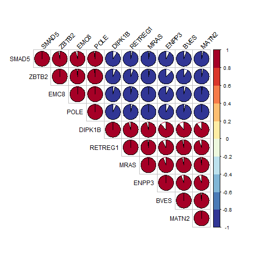
library(cowplot)
cor_plot <- recordPlot()
# 拼图
load("pca_plot.Rdata")
plot_grid(pca_plot,cor_plot,
volcano_plot,heatmap_plot$gtable)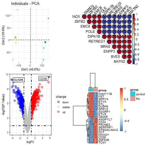
dev.off()## null device
## 1#保存
pdf("deg.pdf",width = 10,height = 10)
plot_grid(pca_plot,cor_plot,
volcano_plot,heatmap_plot$gtable)
dev.off()## null device
## 1GO,KEGG富集分析
rm(list = ls())
load(file = 'step4output.Rdata')
library(clusterProfiler)
library(ggthemes)
library(org.Hs.eg.db)
library(dplyr)
library(ggplot2)
library(stringr)
library(enrichplot)
# 1.GO 富集分析----
#(1)输入数据
gene_up = deg$ENTREZID[deg$change == 'up']
gene_down = deg$ENTREZID[deg$change == 'down']
gene_diff = c(gene_up,gene_down)
#(2)富集
#以下步骤耗时很长,设置了存在即跳过
f = paste0(gse_number,"_GO.Rdata")
if(!file.exists(f)){
ego <- enrichGO(gene = gene_diff,
OrgDb= org.Hs.eg.db,
ont = "ALL",
readable = TRUE)
ego_BP <- enrichGO(gene = gene_diff,
OrgDb= org.Hs.eg.db,
ont = "BP",
readable = TRUE)
#ont参数:One of "BP", "MF", and "CC" subontologies, or "ALL" for all three.
save(ego,ego_BP,file = f)
}
load(f)
#(3)可视化
#条带图
barplot(ego)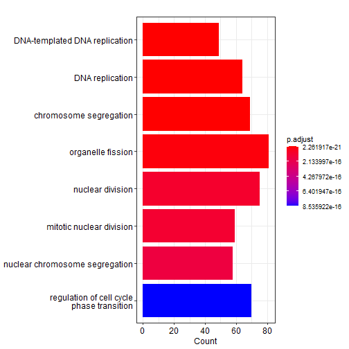
barplot(ego, split = "ONTOLOGY", font.size = 10,
        showCategory = 5) +
facet_grid(ONTOLOGY ~ ., space = "free_y",scales = "free_y") 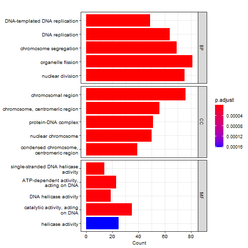
#气泡图
dotplot(ego)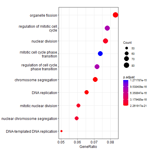
dotplot(ego, split = "ONTOLOGY", font.size = 10,
        showCategory = 5) +
facet_grid(ONTOLOGY ~ ., space = "free_y",scales = "free_y") 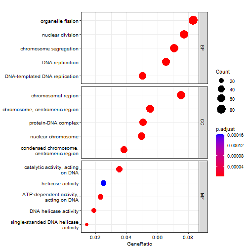
#(3)展示top通路的共同基因,要放大看。
#gl 用于设置下图的颜色
gl = deg$logFC
names(gl)=deg$ENTREZID
#Gene-Concept Network,要放大看
cnetplot(ego,
#layout = "star",
color.params = list(foldChange = gl),
showCategory = 3)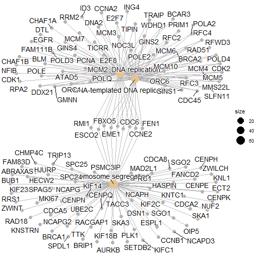
# 2.KEGG pathway analysis----
#上调、下调、差异、所有基因
#(1)输入数据
gene_up = deg[deg$change == 'up','ENTREZID']
gene_down = deg[deg$change == 'down','ENTREZID']
gene_diff = c(gene_up,gene_down)
#(2)对上调/下调/所有差异基因进行富集分析
f2 = paste0(gse_number,"_KEGG.Rdata")
if(!file.exists(f2)){
kk.up <- enrichKEGG(gene = gene_up,
organism = 'hsa')
kk.down <- enrichKEGG(gene = gene_down,
organism = 'hsa')
kk.diff <- enrichKEGG(gene = gene_diff,
organism = 'hsa')
save(kk.diff,kk.down,kk.up,file = f2)
}
load(f2)
##返回空值别紧张,看看帮助文档~ https://mp.weixin.qq.com/s/NglawJgVgrMJ0QfD-YRBQg
#(3)看看富集到了吗
table(kk.diff@result$p.adjust<0.05)
table(kk.up@result$p.adjust<0.05)
table(kk.down@result$p.adjust<0.05)#(4)双向图
# 富集分析所有图表默认都是用p.adjust,富集不到可以退而求其次用p值,在文中说明即可
source("kegg_plot_function.R")
g_kegg <- kegg_plot(kk.up,kk.down)g_kegg#g_kegg +scale_y_continuous(labels = c(2,0,2,4,6))
# 3.能看懂的资料越来越多----
# GSEA:https://www.yuque.com/docs/share/a67a180f-dd2b-4f6f-96c2-68a4b86fe862?#
# 富集分析学习更多:http://yulab-smu.top/clusterProfiler-book/index.html
# 弦图:https://www.yuque.com/xiaojiewanglezenmofenshen/dbwkg1/dgs65p
# GOplot:https://mp.weixin.qq.com/s/LonwdDhDn8iFUfxqSJ2Wew
# 网上的资料和宝藏无穷无尽,学好R语言慢慢发掘~生信技能树-小洁老师课程
原创声明:本文系作者授权腾讯云开发者社区发表,未经许可,不得转载。
如有侵权,请联系 cloudcommunity@tencent.com 删除。
原创声明:本文系作者授权腾讯云开发者社区发表,未经许可,不得转载。
如有侵权,请联系 cloudcommunity@tencent.com 删除。
评论
登录后参与评论
推荐阅读
目录
腾讯云开发者

Copyright © 2013 - 2026 Tencent Cloud. All Rights Reserved. 腾讯云 版权所有
深圳市腾讯计算机系统有限公司 ICP备案/许可证号:粤B2-20090059 ![]() 粤公网安备44030502008569号
粤公网安备44030502008569号
腾讯云计算(北京)有限责任公司 京ICP证150476号 | 京ICP备11018762号